Relational Databases - Design and Principles (Version October 2025)
| |
Copyright 2025 Josef L. Staud |
|
Author: Josef L. Staud |
|
Status: October 2025 |
|
Length of printed text: 42 pages |
|
Origin of the Text |
|
This text (RelDBshortE) is a translation of my German text RelDBkurzD (https://www.staud.info/rmkDoF/rd_t_1.php), which I created in August 2025. The translation into English was carried out with the assistance of DeepL and ChatGPT 5. The final editing was done by me, so the responsibility for the English version rests with me. Both versions can be found on these websites (www.staud.info). |
|
Prof. Dr. Josef L. Staud |
|
Preparation for the web |
|
These HTML pages were created using a program I developed: WebGenerator (version 2021-1). It converts text into HTML pages and is constantly being further developed. The "machine-based" generation makes it possible to instantly re-create the HTML pages after any change in the text. This is now done in two versions: with and without frames. Currently, both versions are offered in parallel for most texts. |
|
Since it is not possible to check all pages after each new creation, it is quite possible that errors may occur somewhere on a "remote" page. I apologize for this and would appreciate any feedback (hs@staud.info). |
|
Copyright |
|
This text is protected by copyright. The rights arising therefrom - particularly the rights of translation, reprinting, public performance, extraction of illustrations and tables, reproduction by other means, and storage in data processing systems - remain reserved, even in the case of utilization in excerpts. Any reproduction of this text, or of parts thereof, is permitted, even in individual cases, only within the limits of the statutory provisions of the Copyright Act of the Federal Republic of Germany of September 9, 1965, as amended. As a matter of principle, reproduction is subject to remuneration. Infringements are subject to the penal provisions of the Copyright Act. |
|
Trademarks and Brand Protection |
|
All common names, trade names, brands, product names, etc. mentioned in this text are subject to trademark, brand, or patent protection or are trademarks or registered trademarks of their respective owners. The reproduction of such names and designations in this text does not entitle the reader to assume that such names are to be regarded as free in the sense of trademark and brand protection legislation and may therefore be used by anyone. |
|
Prof. Dr. Josef L. Staud |
|
|
|
Preface
| |
While this text explains the most important points in the development of relational databases, the following book contains a comprehensive presentation of relational theory (in German): |
|
Staud, Josef Ludwig: Relationale Datenbanken. Grundlagen, Modellierung, Speicherung, Alternativen (2. Auflage). Hamburg 2021 (tredition) |
|
To purchase: https://shop.tredition.com/booktitle/Relationale_Datenbanken/W-1_161508 |
|
Excerpts can be found at https://www.staud.info/rm2/rm_t_1.php |
|
The following collection of exercises serves as a companion piece, so to speak (in German): |
|
DBTraining - Datenbanktraining zu RM, ERM, SQL und OOM. 128 einführende Aufgaben und Lösungen. |
|
This can be found here: https://www.staud.info/AufgabenDBoF/db_t_1.php |
|
It contains exercises and solutions for training the following aspects of databases: |
|
- Modeling relational databases
- Setting up relational databases with XAMPP/mySQL
- Querying and working with databases using SQL
- Setting up a web interface with PHP
- Entity relationship modeling
- Object-oriented modeling according to UML 2.5
|
|
Also with some sample solutions from ChatGPT to see how far current AI has come in solving tasks in this field. |
|
Notes on Text Formatting |
|
When it comes to the elements to be described in data modeling, a starting point and three model levels can be distinguished. The starting point is the application domain to be modeled. The first model level is that of attributes, which are used to describe objects and relationships. The second is the level of the "smallest" elements in the respective approach, which in this case are the relations. The third level is that of the entire data model. In order to increase clarity in the text in this regard, the following typographical specifications have been made: |
|
- Designations of application domains are slightly enlarged, set in small caps and Arial: university, human resources, web shop.
- Designations of data models and databases are displayed in normal size and Arial font: Sales, Zoo, WebShop, Database Systems (market for database systems).
- Designations of relationship names are slightly smaller and set in Arial: Employees, Departments, Projects.
- Designations of attributes are slightly smaller, bold, and set in Arial: Salary, Name, Date. In compound designations, the subsequent term is capitalized again: PersNr (personnel number), BezProj (project designation).
- Attribute values are set in normal size and Courier, e.g., Müller for the Name attribute.
|
|
When naming relations (such as Customers, Invoices, etc.), the plural form is used, since there are always multiple tuples in a relation. |
|
Web Version and Print Version |
|
There is a version of this text for the web (Web Version) and one for print (Print Version). The two differ only in their formal layout. The Print Version, for example, includes a table of contents at the beginning and an index at the end. |
|
|
|
|
|
List of Abbreviations |
|
|
|
| Abbreviation |
Term |
Notes |
| 1NF |
First Normal Form |
Relation without repeating groups, only atomic values. |
| 2NF |
Second Normal Form |
No partial dependencies on parts of a key. |
| 3NF |
Third Normal Form |
No transitive dependencies of non-key attributes. |
| BCNF |
Boyce-Codd Normal Form |
Stronger than 3NF: every determinant must be a candidate key. |
| 4NF |
Fourth Normal Form |
No non-trivial multivalued dependencies other than candidate keys. |
| 5NF |
Fifth Normal Form |
Decomposition so that no join dependencies remain. |
| FD |
Functional Dependency |
Relationship between attributes. |
| KA |
Key Attribute |
Attribute that is part of a key. |
| NKA |
Non-Key Attribute |
Attribute that is not part of a key. |
| PK |
Primary Key |
Unique key of a relation. |
| FK |
Foreign Key |
Key that refers to another relation. |
| |
|
|
|
|
1 Overview: What is this about? |
|
|
|
1.1 Milestones of Database Design |
|
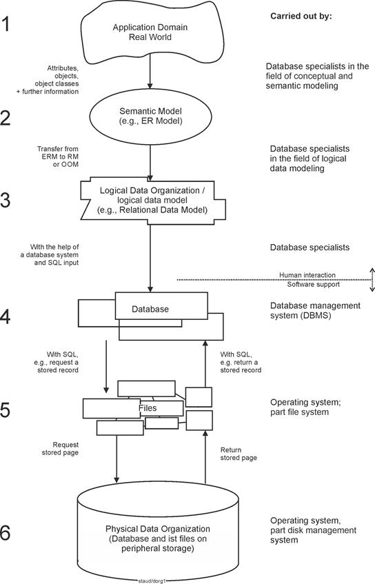
The following figure illustrates the overall process of database design, from the application domain to the database. |
|
|
|
Abbildung 1: Vom Anwendungsbereich zur Datenbank |
|
The following book (in German) covers most of these topics: |
|
Staud, Josef Ludwig: Relationale Datenbanken. Grundlagen, Modellierung, Speicherung, Alternativen (2. Auflage). Hamburg 2021 (tredition) |
|
1.2 Contents |
|
- This text is a summary of the book mentioned above. It provides a concise overview of the most important topics shown in the figure:
- Chapter 3 deals with relations - data tables with a specific structure that are of central importance.
- Chapter 5 explains how relationships are implemented in relational data modeling.
- Chapter 6 shows how the relational theory is used to optimize the data model. The tool for this purpose consists of six normal forms. The focus - due to their great practical relevance - is on the first three: 1NF, 2NF, and BCNF.
- Chapters 7 through 11 demonstrate how central semantic patterns are implemented in relational data models: "semantics seeks syntax". These range from handling instance and type information to generalization/specialization, aggregation, composition, and relationship properties.
- Chapter 12 summarizes the rules for developing relational data models.
- Chapters 13 through 14 use a sample case (Invoices) to illustrate how to create a database using SQL.
|
1.3 Target Audience |
|
This text is intended for beginners in the field of database design. It is particularly suitable for students at colleges and universities, learners in community colleges or vocational programs, as well as professionals seeking to gain knowledge of databases through corporate training or certification courses. |
|
The material provides a concise introduction to the fundamental concepts of database design and supports both academic study and practical application in projects and professional settings. |
|
2 Application Domains |
|
At the beginning of database development, the scope of the application domain must be clarified. What data should be recorded in the database, what evaluations should be possible with the data, and what business processes should be supported? In database theory, this stage is referred to as conceptual modeling. Only the most essential aspects are outlined here; for a more detailed discussion, see https://www.staud.info/rm2/rm_t_1.php#Kapitel4 and the literature listed there. |
|
The section of the real or fictional world that is to be recorded in the database is therefore called the application domain. The very simple database view of application domains initially only perceives objects with their attributes (employees of a company; departments of a company) and relationships between the objects (employees work in departments). |
|
Other terms have also been used in this context, such as slice of reality, universe of discourse, and subject area. |
|
Objects |
|
Objects here refer to objects in the colloquial sense. In other words, everything we perceive and assign properties to. Of these properties, those that are attributes are considered (employees have a surname, first name, a certain age, etc.). See below. |
|
In object-oriented theory, the concepts of objects and object classes (see below) are also used. There, too, they are carriers of attributes, but also of methods and much more. They are the starting point for the theoretical explanations. See https://www.staud.info/leitOO.php for an introductory presentation. |
|
If you want to add a little theoretical twist, you could define objects as elements of our perception to which we can assign descriptive attributes and at least one identifying attribute. In other words, to put it simple: |
|
Objects are all perceived phenomena that can be identified and described by attributes. |
|
Attributes |
|
Attributes therefore describe the properties of objects. For the employees of a company, for example |
|
- Employee ID (EmpID)
- Employee Name (EmpName)
- First name (FirstNname)
- Last Name (LastName)
- Date of hire (HireDate)
- Birthday (BirthDate)
|
|
How are these attributes structured? They have a name, various attribute values, and objects or relationships they describe. Let's look at a few examples: |
|
- Widmer, Maier, etc. as names of employees in a company
- Black, white, gray, red, etc. as colors of cars
- Male, female as the gender of cats
- 126 as a blood sugar measurement for diabetics
- 5, 10, 20, 50, ... as the duration of marriages in years
- 5000.00 euros or another positive amount as the salary of employees
- 10050, 10051, ... as ID numbers of employees
- 1.7 or another number between 1 and 5 as a grade in university exams
|
|
All underlined words are examples of attribute names. All words and numbers in italics are examples of attribute values, i.e., values that an attribute can take on. The number of values must be at least 2 (for example, for gender), it can include a few (color of cars) or many (names, measured values). |
|
Attributes can take on certain values, which are called attribute values. |
|
All words in bold denote objects and relationships (in the most general sense) and, after some modeling steps, relations. They are described by attributes and their values. Objects and relationships must be specified, otherwise it is not clear what the attributes refer to. This relationship between attribute names, attribute values, and objects/relationships is fundamental and can be stated as followas: |
|
- Attributes have a specific set of attribute values.
- Attributes are assigned to objects/relationships.
- An object has a valid attribute value for each attribute, sometimes even several.
|
|
For a more comprehensive description, see https://www.staud.info/rm2/rm_t_1.php#Abschnitt3.4. |
|
Object class |
|
Objects that share the same structure - that is, objects with the same attributes, the same key, and the same descriptive attributes - are grouped together into object classes. The above attributes could then describe an object class Employees. A single object would then be, for example, Andrea Maier, born on October 10, 2001, hired on December 20, 2022, with employee number 1008. |
|
If you want to define and delimit the scope of application for the database to be created, you must identify the object classes that occur in it with their attributes and the relationships between them. |
|
How can object classes be distinguished from one another? The following rule is useful: all objects that are identified by a key and described by additional attributes belong together and constitute an object class. |
|
For example, if the following attributes have been collected for employees ... |
|
- Employee ID (EmpID)
- Last Name (LName)
- First name (FName)
- Date of hire (HireDate)
- Date of birth (DOB)
- Department name (DeptName) in which he or she works
- Department head (DeptHead)
- Department location (DeptLoc)
... one must recognize that there are in fact two object classes: |
|
- The objects in Employees are identified by EmpID and described by LName, FName, HireDate, DOB, and DeptName.
- The objects in Departments are identified by DeptName and described by DeptHead and DeptLoc.
- The relationship between Employees and Departments is established through the attribute DeptName in the Employees relation.
|
|
Relationships |
|
Relationships are defined here as follows: |
|
- They exist between object classes or objects. For example, if there are the object classes Employees and Departments, then there is the relationship Employee works in Department.
- They are based on attributes; in the above example, the personnel number (1008) is linked to the department name (HR; Human Resources).
|
|
For a detailed presentation, see https://www.staud.info/rm2/rm_t_1.php#Kapitel6 (in German). For a fundamental discussion of relationships in all modeling approaches, see https://www.staud.info/Beziehungen/bz_t_1.php (in German). |
|
Just as for objects, classes are also formed for relationships. Here, however, it is usually the case that more than one attribute is required to identify each relationship. |
|
|
|
|
3 Relations |
|
|
|
3.1 From classes to relations |
|
In the next step, each of the object and relationship classes found is recorded in a table. This is done as follows: |
|
- The attribute designations are listed at the top of the columns.
- Below this, the attribute values that describe an object or a relationship are listed line by line, sorted according to the attribute order in the header. In relational theory, these lines are called tuples.
|
|
Let us consider the above example of the object class Employees. The table can (in a simplified and abstracted form) look as shown below. One of the attributes must have an identifying character; here it is the employee number. It is called the key (of the relation) and is marked with a hash sign (more on this below). For the object class Employees, a table like the following is therefore created: |
|
Table Employees |
|
| #EmpID |
LName |
FName |
HireDate |
DOB |
| 1001 |
Müller |
Karolin |
March 1, 2010 |
May 14, 1985 |
| 1010 |
Jäger |
Rolf |
October 1, 1990 |
September 21, 1959 |
| 1020 |
Wilkens |
Jenny |
January 1, 2007 |
March 23, 1970 |
| 1030 |
Forster |
Charles |
October 1, 2010 |
July 31, 1985 |
| 1005 |
May |
Lisa |
July 1, 2009 |
September 21, 1970 |
| 1040 |
Winter |
Angelika |
February 1, 2007 |
September 17, 1965 |
| 1007 |
Miller |
Igor |
May 1, 2008 |
November 22, 1962 |
| 1090 |
Stepper |
Rolf |
July 1, 2013 |
April 15, 1974 |
| |
On key notation: In this text, I use the hash sign (#) to mark the primary key of a relation rather than underlining, since underlining is reserved in relational database theory for foreign keys. In ER modeling, by contrast, primary keys are conventionally indicated by underlining. |
|
Let's look at a second example, the object class Departments with the attributes: |
|
- Department name (DeptName)
- Head of department (DeptHead)
- Department location (DeptLoc)
|
|
This results in the following table. |
|
Table Departments |
|
| #DeptName |
DeptHead |
DeptLoc |
| HR |
Summer |
Munich |
| IT |
Winter |
Ulm |
| AC |
Müller |
Munich |
| SA |
Stepper |
Munich |
| |
HR=Human Resources, IT=Information Technology, AC=Accounting, SA=Sales |
|
Now for the object class of the Projects. For these, a name (ProjName), the start date (StartDate), the duration in month (Duration), and the budget (Budget) are recorded. |
|
Table Projects |
|
| #ProjName |
StartDate |
Duration |
Budget |
| Delivery portal |
10/01/2013 |
60 |
200 |
| Ind4p0 |
01/01/2014 |
48 |
600 |
| BPM |
04/01/2013 |
48 |
150 |
| |
Finally, there is the PC object class. It describes the PCs used in the company. |
|
Table PCs |
|
| #PCID |
PCName |
Type |
| pc2012 |
HP xyz |
Desktop office |
| pc3015 |
Acer zyx |
Desktop dev |
| Pc1414 |
HP Envy xyz |
Laptop |
| |
|
|
Tables of this kind, provided they meet certain criteria, are referred to as relations. At this level of modeling, a relation is simply a table that follows specific rules and serves to describe either a class of objects or a class of relationships. |
|
3.2 Properties and Representation of Relations |
|
The following are the properties that a table must fulfill in order to qualify as a relation: |
|
|
(1) Each row (also called a "tuple") describes an object (or a relationship), and the table as a whole describes the object class or relationship class.
|
|
|
(2) Each column has as its heading the name of an attribute, and beneath it the attribute values that describe the respective object (or relationship).
|
|
|
(3) A relation always has a key, which can consist of more than one attribute, and at least one descriptive attribute.
|
|
|
(4) No two tuples are identical, i.e., each tuple describes a different object.
|
|
|
(5) Exactly one attribute value is recorded at the intersection of each row and column, no more. This makes the table a flat table .
|
|
Comment on (1): This is correct at the beginning of the creation of a data model. Later, when any redundancies in the model designs are eliminated - keyword normalization (see chapters 7 - 13 in [Staud 2021]) - the attributes of an object may be distributed across several relations and thus across several tuples. |
|
Comment on (2): This is how the tables were introduced above. |
|
Comment on (3): Because a key alone does not carry much informational content. |
|
Comment on (4): This can also be justified with the mathematical derivation of relational theory, cf. [Staud 2006, section 3.22]. However, it is also sufficient to realize that two tuples of a relation with the same key and the same attributes do not make sense, because they describe the same object or the same relationship. |
|
Comment on (5): The latter property is particularly important in relational theory and also causes some difficulties when setting up a database (when creating the data model). Specifically, it means that a table must be reorganized if more than one value of an attribute can be assigned to an object. This situation is referred to as multiple entriesor repeating groups (repeating groups). If, for example, the attribute ProjName (project name) were also included in the following figure (projects in which the employees are working), multiple entries could occur if an employee is working on several projects. |
|
The tables introduced above meet all these requirements and can therefore be continued as relations. |
|
Focus: Relations as flat tables |
|
Relational theory is based entirely on these relations and only on them, and relational database systems (RDBS) are based on this in turn. All object and relationship classes are represented exclusively by relations and only by them. |
|
Relational database systems are also fully tailored to this type of information. They have commands for setting up these relations, defining attributes, etc. They also make it possible to join relations, evaluate them, and perform further operations. |
|
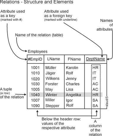
The following figure shows how relations can be represented as tables and how they are structured. Each relation has a name, in this case Employees. The top row contains the names of the attributes. Keys (identifying attributes) and foreign keys are already marked here; they are explained below. The rows beneath contain the values of the attributes specified in the header. In relational theory, these lines are called tuples. A tuple thus describes an object or a relationship (see the next section). The attributes that are foreign keys are used for linking, see the definition above and the more detailed description in the next section. |
|
Version1: Didactically motivated graphical representation of relations |
|
|
|
Figure 3.2-1: Structure of relations. |
|
Departments:
HR: Human Resources
IT: Informatin Technology
AC: Accounting
SA: Sales
Attributes:
EmpID: Employee ID
LName: LastName
FName: First Name
DeptName: Department Name |
|
Version 2: Textual Representation of Relations |
|
In addition to this graphical representation, the following textual notation is also used for relations: |
|
Relation name (#A1, A2, A3, ...) |
|
Here, A1, A2 etc. stand for the attributes of the relation. The hash symbol (#) indicates the key attribute, while underlining indicates the foreign key. For the example above, this means: |
|
Employees (#PersNo, Name, VName, ..., EmplID) |
|
Multiple attributes in the key. It can happen that the key of a relation consists of several attributes, e.g., in certain relationships (see the next section). In this case, the key attributes (here A1 and A2) are enclosed in parentheses: |
|
Relation name (#(A1, A2), A3, A4, ...) |
|
SQL. If an attribute name needs to be supplemented with information about its relation (e.g., in SQL, where this is sometimes essential), the relation name is placed in front: |
|
Relation name.Attribute name |
|
For example, Employees.Name or Departments.DeptHead. |
|
Here are all of the above relations for the application domain Employees in this textual representation: |
|
Employees (#EmpID, LName, FName, HireDate, DOB) |
|
Departments (#DeptName, DeptHead, DeptLoc) |
|
Projects (#ProjName, StartDate, Duration, Budget) |
|
PCs (#PCID, PCName, Type) |
|
The keys mean: |
|
- EmpID: Employee ID
- DeptName: Short name of the department
- PCID: Inventory number of the PC
- ProjName: Name of the project
|
|
Version 3: Correct graphical representation of relations in data models |
|
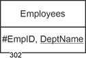
The correct graphical representation of relations in data models is as shown in the following figure. In a rectangle, the relation name is specified in the upper half, with the keys and foreign keys (and only these) below. This representation is required when entire data models (i.e., many relations with their links) are to be represented (see chapters 7 to 13 and, in particular, the numerous examples in chapters 16 and 17 of [Staud 2021]; excerpts: https://www.staud.info/rm2/rm_t_1.php). |
|
Foreign keys are used to link different relations with each other and are therefore of great importance in relational modeling. They are explained in the next chapter. |
|
|
|
Figure 3.2-2: Graphical representation of relations |
|
Examples from the employee application domain |
|
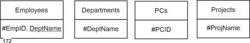
The example introduced in this section deals with the application domain of employees of a company (in simplified form). Here is the graphical representation of the four relations. |
|
|
|
Figure 3.2-3: Relationships from the application domain Employees |
|
So much for the relations in the example and their representation. The following table summarizes the basic concepts of relations. The concepts from the database theory discussion are supplemented by informal concepts, where these exist. |
|
Relational terminology |
|
| Informal |
Formal |
| Table |
Relation |
| Row |
Tuple |
| Property - Designation |
Attribute designation |
| Property - Value |
Attribute values |
| |
3.3 Why are these tables called relations? |
|
The term relation is associated with relationship. This is why some authors confuse the table name with the relational link, which also represents a relationship. In relational database theory, however, relation refers to the tables described above. This comes from the originators of relational theory, Codd and Date. If we take the term relationship as a starting point, then the idea was to express that the attributes of a relation are closely related. They each describe an object or a tuple. |
|
In particular, relations are not the links between tables, as is often stated in popular literature. |
|
See, for example, the authors: |
|
Codd 1970
Codd, E. F. A relational model of data for large shared data banks, in: Communication ACM, ACM, Vol. 13, No. 6, pp. 377-387, June 1970 |
|
Date 1990
Date, C.J.: An Introduction to Database Systems. Volume I (5th edition), Reading et al. 1990 |
|
3.4 Attributes and functional dependencies |
|
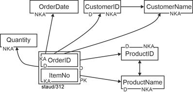
The following discussion is based on the relation Orders, which records standard business orders and has the following structure: |
|
Orders (#(OrderID, ItemNo), OrderDate, CustomerID, CustomerName, ProductID, ProductName, Quantity) |
|
OrderID: order number
ItemNo: item (line) number
OrderDate: order date
CustomerID: customer Number
CustomerName: customer name
ProductID: product number
ProductName: product Description
Quantity: number of items per line |
|
Attributes can take on different roles in relational data models and are interrelated. Specifically: |
|
- They can identify individual tuples. In this case, they are called key. If there are several keys, one of them is the primary key (PK). Keys may also be composed of multiple attributes.
- If they are part of a composite key, they are called key attributes(KA).
- Attributes that are not part of any key are called non-key attributes (NKA).
- Attributes can be functionally dependent on each other. This means that one attribute (e.g., EmployeeID) can be used to infer another (e.g., Name). Any attribute on which others are functionally dependent is called a determinant attribute (D). In the example above, EmployeeID is a determinant attribute, since every key is, of course, also a determinant attribute. However, there are also determinant attributes that are not keys. More on this below.
|
|
If the attributes of a relation are represented as labeled rectangles and the functional dependencies are entered as arrow lines between the attributes, the result is a diagram like the one below, which says a lot about the internal structure of the relation. It is called an FD diagram. The roles of the attributes are also noted in the diagram. |
|
|
|
Figure 3.4-1: Functional dependencies of the relation Orders |
|
KA: key attribute.
NKA: non-key attribute
D: determinant attribute
PK: primary key |
|
3.5 Full and Non-Full Functional Dependency |
|
If the determinant attribute consists of several attributes, and if some of these attributes are not required for a given functional dependency, then the functional dependency is non-full. Conversely, if all attributes of the determinant are necessary for the functional dependency under consideration, it is called a full functional dependency. |
|
Example: |
|
Consider the relation Orders: |
|
Orders(#OrderID, CustomerID, CustomerName, City) |
|
- Functional dependency: (OrderID, CustomerID) => CustomerName
|
|
Here, the dependency is non-full, because CustomerID alone is sufficient to determine CustomerName. OrderID is not needed. |
|
- Functional dependency: (OrderID) => OrderDate
|
|
This is a full functional dependency, because OrderID alone is necessary and sufficient to determine OrderDate. |
|
Cf. [Staud 2021, Chapter 8] for a detailed presentation in German (https://www.staud.info/rm2/rm_t_1.php#Kapitel9). |
|
3.6 Anomalies |
|
Let us once again consider the relation Orders: |
|
Orders (#(OrderID, ItemNo), OrderDate, CustomerID, CustomerName, ProductID, ProductName, Quantity) |
|
Relations may appear to be neat tables and still exhibit faulty structures. This happens when the rules for correct relations defined in Section 2.2 are not followed. The above relation Orders illustrates this, filled with fictitious data for demonstration purposes. |
|
This relation records information about orders. OrderID identifies the order, while ItemNo identifies the individual line items of an order. Each line item refers to a product, which is named by ProductName and additionally identified by ProductID. Quantity specifies how many units of the product are included in the line item. The attribute CustomerID identifies the customer to whom the order belongs. The customer names (CustomerName) are not unique. |
|
Orders_1NF |
|
| OrderID |
ItemNo |
ProductID |
ProductName |
Quantity |
OrderDate |
CustomerID |
Customer-Name |
| 0001 |
1 |
9901 |
Laser Printer x |
1 |
06/30/22 |
1700 |
Miller |
| 0001 |
2 |
9910 |
Toner xyz |
3 |
06/30/22 |
1700 |
Miller |
| 0001 |
3 |
9905 |
Paper abc |
5,000 |
06/30/22 |
1700 |
Miller |
| 0010 |
1 |
9905 |
Paper abc |
30,000 |
07/01/24 |
1201 |
Sanders |
| 0010 |
2 |
9910 |
Toner xyz |
1 |
07/01/24 |
1201 |
Sanders |
| 0011 |
1 |
9901 |
Laser Printer x |
1 |
07/02/25 |
1600 |
Johnson Inc. |
| 0011 |
2 |
9911 |
Ink Cartridge x |
20 |
07/02/25 |
1600 |
Johnson Inc. |
| 0011 |
3 |
9905 |
Paper abc |
5,000 |
07/02/25 |
1600 |
Johnson Inc. |
| 0011 |
4 |
9906 |
InkJet Printer y |
2 |
07/02/25 |
1600 |
Johnson Inc. |
| 0012 |
1 |
9998 |
Monitor z |
1 |
07/04/23 |
1900 |
Maxwell LLC |
| ... |
... |
... |
... |
... |
... |
... |
... |
| |
Key: #(OrderID, ItemNo) |
|
It is easy to see that the two attributes OrderID and ItemNo form the key of the relation, because the combination of their values uniquely identifies each tuple (row). |
|
Let us now turn to the deficiencies of this "relation". The following three anomalies have been described in the literature: update anomaly, insertion anomaly, and deletion anomaly. |
|
Update Anomaly |
|
One update, several tuples to change. An update anomaly occurs when changing a single piece of information requires modifying multiple tuples. This is fundamentally undesirable. The consequence is that, when updating a value, the number of tuples that need to be changed is not known in advance. In the worst case, the entire relation must be searched. The cause of such a structure is that the same piece of information is stored multiple times in the database. |
|
In the example above: If product names are changed, e.g. ProductID 9901, previously called Laser Printer x, is now called HP Laser Printer Series 5, then the product name must be changed not only in one tuple, but in several. It is easy to overlook some occurrences. |
|
The same applies to OrderDate. If this value must be changed for some reason, it must be changed in multiple tuples. The same issue holds for CustomerName. If the name of customer 1700 changes from Miller to Miller amp; Paul, multiple changes are again required. |
|
It is clear what causes this anomaly: a violation of the central rule of database design, namely that the database should be designed so that each piece of information is stored only once. |
|
Insertion Anomaly |
|
Insertion blocked. Redundancy also causes difficulties when inserting data, leading to insertion anomalies. Such an anomaly occurs when a new (still incomplete) tuple cannot be entered into the relation - for example, because one of the missing attributes is a key attribute. This may also happen with foreign keys. |
|
The anomaly is based on the rule that a tuple can only be entered into the relation if values for the key attributes (the attributes forming the key) are present (see Section 5.9 on the requirement of entity integrity). |
|
In the example above: If we want to add new products with ProductID and ProductName, we cannot record them in the relation until they appear in at least one order with an Item Number. Otherwise, entry is impossible, since no key attribute would exist. The same applies to OrderDate: it can only be recorded once the first item of the order is known. The same holds for CustomerID and CustomerName. |
|
The cause of this anomaly lies in the fact that the relation combines several different "things": the object classes Orders, Products, and Customers, as well as the relationship class Orders - Customers. This structural weakness is addressed using the concept of functional dependencies (see the next chapter). |
|
Deletion Anomaly |
|
Problems when deleting. The last anomaly describes problems that arise from redundancies when deleting records. A deletion anomaly occurs when deleting information that concerns only part of a tuple also removes other attribute values. |
|
In the example above: If we delete order 0012, which has only one item, we also lose the information that product Monitor z has the ProductID 9998. |
|
Again, the cause is the mixing of several object and relationship classes in a single relation. |
|
Goal |
|
Bringing order to the "attribute heap". What is the goal of identifying and eliminating anomalies? Even these very simple examples show the purpose of the three anomalies: they help clarify which attributes should be grouped together and which should be separated. They thus bring order to the "heap of attributes and characteristics," the so-called universal relation, that arises at the beginning of every modeling effort. |
|
While 1NF ensured that attributes remain together if their values can be assigned to objects so that each value is combined with exactly one other, the situation here is different. Now the goal is to group attributes so that, together with a key, they form a "homogeneous" block: they describe exactly the objects identified by the key, and no others. |
|
This is achieved by eliminating the redundancy inherent in such relations. Its removal also clarifies the arrangement of attributes in the relation. A very useful tool for clarifying the internal structure of relations are functional dependencies, which will be discussed in the next chapter. |
|
3.7 What happens next? |
|
Defining the relationships is the first important step. After that, the following must be done: |
|
|
(1) Produce flat tables. That is, ensure that for each value of the key, there is exactly one value for every non-key attribute (NKA). Above, it was described how the initial designs of relations are created. Example: Employees with #PersNr and Name, FirstName. ProjectParticipation with #(PersNr, ProjBez), StartDate, Role. For each such relation, it must be ensured that for every single key value, there is exactly one value for each non-key attribute. Because: In relational databases, an attribute has exactly one value per object. This brings the relations into First Normal Form (1NF).
|
|
|
(2) Ensure that the attributes selected for a relation truly describe all objects or relationships in the relation. In other words, the attribute must be applicable to all objects so that no semantically induced null entries (cf. [Staud 2021, p. 183f]) occur. Example: ProgrLang (programming language mastered) in a relation of employees that also includes non-programmers.
|
|
|
(3) Refine the relationships that arise from the steps above (primary key/foreign key relationships). The guiding principle here is the general rule: all relations must be interconnected, at least indirectly (loose coupling). This does not mean that every relation must be directly connected to every other, but rather that each relation must be linked to the overall model.
|
|
|
(4) Specify the relationships found with regard to the further normal forms. This usually results in further key/foreign key relationships. The decompositions within the process of normalization must not lead to any loss of information. That is, care must always be taken to ensure that, through relational connections along keys and foreign keys, the information present in the original relation remains preserved.
|
|
|
(5) Clarify and incorporate additional relationships into the data model. This concerns semantically justified relationships that do not follow directly from the constellation of attributes or from the modeling method itself.
|
|
|
(6) Identify and create generalization/specialization (Gen/Spec) patterns.
|
|
|
(7) Examine and incorporate further patterns (e.g., entity/type, aggregation, composition).
|
|
|
(8) Clarify and model temporal aspects, including those omitted in the initial requirements specification.
|
|
The methods and procedures for these steps are described in the following chapters. |
|
4 Patterns everywhere |
|
Here, patterns refer to recurring structures in relational data models. Patterns can be distinguished between those that arise from the method and those that arise from the semantics of the application domain. |
|
Methodological patterns - "Method seeks Syntax " |
|
These are, for example, those that result from normal forms. Their implementation frequently leads to decompositions that must be implemented and managed. For example, a new additional relation must be created if there are multiple entries in the initial relation. The basis for this are the relational links, from 1:1 to n:m relationships. For a more detailed description, see Chapter 5 in [Staud 2021] and |
|
www.staud.info/rm2/rm_t_1.htm#Kapitel6 |
|
Semantic patterns - "Semantics seeks Syntax" |
|
These are patterns that result from the capture and modeling of semantic relationships. For example, employees work in departments, employees have assigned PCs, lecturers hold classes. These are also realized via relational links. For a basic description of the implementation of relationships in data models, see |
|
https://www.staud.info/Beziehungen/bz_t_1.php (in German) |
|
|
|
|
|
5 Relationships and Cardinalities |
|
In the following chapters it will be shown that, in the course of data modeling, numerous individual relations arise that are interconnected and that, in the context of evaluation, may need to be linked with one another. The methodological foundations for this are explained here. |
|
The relationships here are relationships between the tuples of different relations. These are expressed by key/foreign key combinations. The following values are distinguished: |
|
- 1:1. One tuple from one relation is related to exactly one tuple of the other. Example: Invoices and Customers.
- 1:n. One tuple of one relation is related to several of the others. Example: Invoice headers and invoice line items.
- N:m. One tuple of one relation is related to several of the others and vice versa. Example: Projects and Employees.
|
|
These values are called cardinalities. |
|
Here, they are further specified by indicating whether optional participation is also possible and the maximum number of participants. These min/max specificationsare useful in terms of database technology as they describe the semantics of the model more precisely. They consist of two values separated by a comma, with the first value expressing the minimum participation and the second value expressing the maximum participation. This notation is borrowed from object-oriented theory. |
|
This results in the following variants of relationship cardinalities: |
|
For the 1:1 cardinality |
|
- 1,1 : 1,1
- 0,1 : 1,1
- 1,1 : 0,1
- 0,1 : 0,1
|
|
For the 1:m cardinality |
|
- 1,1 : 1.n
- 0,1 : 1.n
- 1,1 : 0.m
- 0,1 : 0,n
|
|
For the n:m cardinality |
|
- 1.n : 1.m
- 0,n : 1.m
- 1,n : 0,m
- 0,n : 0,m
|
|
|
|
5.1 Cardinality 1:1 |
|
For more information, see [Staud 2021, Section 5.3] and https://www.staud.info/rm2/rm_t_1.php#Kapitel6 (in German) |
|
If the semantics are such that a tuple of one relation is linked to one of the other and vice versa, then the cardinality is 1:1. As an example, the relations Employee and PC can be taken from a personnel database if the semantics specify that each employee is assigned exactly one PC and each PC is used by only one employee. |
|
Here, too, the min/max specifications can be used to clarify: |
|
- 1,1 : 1,1 means that each tuple of one relation is linked to exactly one of the others and vice versa (employees - addresses).
|
|
In the example: An employee is assigned exactly one PC and each PC is assigned to only one employee. |
|
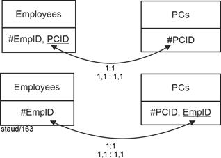
Relational theory allows two solutions for this, which are shown in the following figure. One of the two relations "delivers" its key as a foreign key to the other. This ensures that the semantics and the link are correctly anchored in the database. Here is the graphical representation. |
|
|
|
Figure 5.1-1: Two equally valid methodological solutions for:
Cardinality 1:1 with min/max specification 1,1 : 1,1 |
|
Now for the other variants: |
|
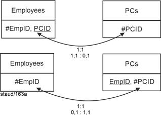
- 1,1 : 0,1 or 0,1 : 1,1 means that the key from the relation with the optional attribute (minimum 0) is entered into the other relation as a foreign key.
|
|
In the example: If not every PC is assigned to an employee, InvPC becomes the foreign key in Employees. If not every employee has a PC, PersNr becomes the foreign key in PC. See the following figure for the graphical representation. |
|
|
|
Figure 5.1-2: Cardinality 1:1 with min/max values 0,1 : 1,1 or 1,1 : 0,1 |
|
The last variant: |
|
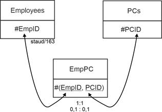
- 0,1 : 0,1 means that participation in the relationship is optional in both relations. Relational theory requires the creation of a separate relation with a key consisting of the keys of the two relations.
|
|
In the example: The new relation EmpPC (employees/PC) receives the key #(EmpID, PCID). Each foreign key establishes the connection to the relation in which it is a key. See the following figure for the graphical representation. |
|
|
|
Figure5.11-3: Cardinality 1:1 with min/max values 0,1 : 0,1 |
|
Source of error to be avoided: The above is not a junction relation as it occurs in n:m relationships below. |
|
5.2 Cardinality 1:n |
|
See https://www.staud.info/rm2/rm_t_1.php#Abschnitt6.5 for a more detailed presentation (in German) |
|
1,1 : 1.n. The first variant is the case that comes to mind when one thinks of cardinality 1:n. In reality, however, it is rather the exception. In this case, every tuple of the two relations participates in the relationship. |
|
In the example of departments/employees, this means - quite understandably - that each department has employees (at least one) and each employee is in a department. Accordingly, the key of Departments can be stored in the employee relation: |
|
Departments (#DeptName, DeptHead, Location) |
|
Employees (#EmpID, LName, Fname, HireDate, DOB, DeptName) |
|
This does not work the other way around. The key of Employees in Departments would lead to multiple entries, which is prohibited for relational data models. The following figure shows the implementation in a data model. |
|
|
|
Figure5.21: Relational link for Departments / Employees with the min/max specifications 1,n : 1,1 |
|
Cardinality: 1:n
Min/max specifications: 1,n : 1,1
Semantics:
- A department has at least one employee.
- An employee is assigned to exactly one department. |
|
1,1 :0,n. This variant means that the foreign key must be stored in the relation with mandatory participation. This is then the one from which each tuple enters exactly one relationship. In this example, it means that there are departments to which no employees are (yet) assigned, e.g., because they have been set up but not yet staffed. On the other hand, all employees participate in the relationship. Therefore, the implementation here can be the same as in the previous case. |
|
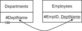
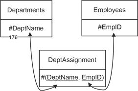
0,n : 1,1. New relation. This variant means that the foreign key would have to be stored in the relation where each tuple could enter into multiple relationships. However, this is not possible because it would result in multiple entries. This creates the need to set up a new relation (department affiliation; DeptAssignment) for the relational relationship. |
|
0,1 : 0,n. The same applies here: since optional participation exists on both sides, the foreign key cannot be placed in either relation without creating inconsistencies. A new relation must therefore be established. |
|
Departments (#DeptName, DeptHead, Location) |
|
Employees (#EmpID, LName, Fname, HireDate, DOB) |
|
DeptAssignment (#(DeptName, EmpID)) |
|
The new relation has a composite key consisting of the two foreign keys. The following figure shows the resulting small data model. |
|
|
|
Figure 5.2-2: Relational link for Departments / Employees and the min/max values 0,1 : 1.n and 0,1 : 0,n |
|
Cardinality: 1:n
Min/max specifications: 0,1 : 1.n or 0,1 : 0,n.
Semantics 0,1 : 1.n:
- A department has no employees, one employee, or several employees assigned to it.
- An employee is assigned to none or exactly one department.
Semantics 0,1 : 0,n:
- One or more employees are assigned to a department ("at least one").
- An employee is assigned to none or exactly one department. |
|
5.3 Implementation of n:m |
|
See https://www.staud.info/rm2/rm_t_1.php#Abschnitt6.6 for a more detailed presentation (in German) |
|
A cardinality of n:m means that several tuples of one relation are related to several tuples of the other relation, and this works in both directions. |
|
Realization of the link through a junction relation |
|
The solution here always consists of creating a new relation, as transferring a key to the other relation would result in multiple entries. In the new relation, called the junction relation, the two keys of the relations to be linked together form the key and are each foreign keys individually. Here, consideration of the various min/max specifications reveals no need for special solutions. In all variants, the join relation provides a problem-free link. |
|
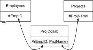
Example: Project Participation. This is the case with a "Project Participation" relationship between employees and projects in an organization. An employee can work on several projects, and a project can have several employees assigned to it: |
|
Employees (#EmpID, LName, FName, HireDate, BOD) |
|
Projects (#ProjName, StartDate, Duration, Budget) |
|
The junction relation is as follows: |
|
ProjCollab (#(EmpID, ProjName)) |
|
Together with the initial relations, this results in a small data model that captures the n:m relationship in all min/max variants. |
|
|
|
Figure 5.3-1: Relational link for employees/projects and cardinality n:m |
|
For clarification, here are the specific semantics: |
|
- 1,n : 1,m: An employee is assigned to at least one project. A project has at least one assigned employee.
- 1,n : 0,n: An employee is assigned to none, one, or several projects. A project has at least one assigned employee.
- 0,n : 1,m: An employee is assigned to at least one project. A project has no, one, or several assigned employees.
- 0,n : 0,m: An employee is assigned to none, one, or several projects. A project has none, one, or several assigned employees.
|
|
The key here is always composed of two attributes. Both attributes must have entries for each tuple. |
|
6 Normal forms |
|
This chapter addresses the optimization of the initial design with respect to the requirements of relational theory. In this process, relations are decomposed as dictated by the method, resulting in methodological patterns. Since there is often a need to reassemble the data for specific evaluation purposes, linkages are introduced. These are implemented through primary keys and foreign keys. |
|
From now on, each relation's normal form will be indicates. For example: Employees_1NF, Employees_2NF, and so on, or Employees_UN. UN stands for unnormalized (not in 1NF). |
|
|
|
6.1 First normal form - 1NF |
|
For a more detailed description, see https://www.staud.info/rm2/rm_t_1.php#Kapitel8 (in German) |
|
Above, in the definition of relations, it has already been described that relations are flat tables (i.e., without multiple entries) with the properties listed. Then they are also in first normal form (1NF). As long as they do not fully meet these properties, they are referred to, linguistically not entirely correctly, as unnormalized relations. |
|
Definition of 1NF |
|
A relation is in 1NF if it has no duplicate entries. |
|
Let's consider the following example. |
|
The Prod_UN relation abstractly and simply records manufacturers of database systems, along with the database systems and address details. |
|
Producer_UN |
|
| #ProducerName |
DBSystemName |
City |
Street |
Country |
| Microsoft |
FoxPro, ACCESS |
AAA |
... |
... |
| CA |
IDMS, Datacom |
CCC |
... |
... |
| Oracle |
Oracle |
DDD |
... |
... |
| ... |
|
|
|
|
| |
CA: Computer Associates / Broadcom
ProducerName = name of the vendor/manufacturer of a database system
DBSystemName = name of the database system
Country = address information of the producer |
|
Tuple multiplication |
|
One way to bring a non-normalized relation into 1NF is by duplicating tuples. This means that a separate tuple is created for each multiple entry. In this case, it results in the following solution: |
|
Producer_1NF |
|
| ProducerName |
#DBSystemName |
City |
Street |
Country |
| Microsoft |
FoxPro |
AAA |
... |
... |
| Microsoft |
ACCESS |
AAA |
... |
... |
| CA |
IDMS |
CCC |
... |
... |
| CA |
Datacom |
CCC |
... |
... |
| Oracle |
Oracle |
DDD |
... |
... |
| ... |
|
|
|
|
| |
It is important to note the new key. With the semantic assumption that each database system is produced by exactly one company, the new key is #DBSystemName. If, however, the semantics were such that several companies could jointly produce a database system, then the key would be #(Producer_UN, DBSystemName). |
|
As can be seen, the above procedure leads for the first time to redundancies in the non-key attributes (NKA). These redundancies, however, will be eliminated in the next step. If one wants to avoid this temporary occurrence of redundancies, one must choose one of the methods presented in the next two sections. These methods, however, require a deeper understanding of relational relationships. |
|
Decomposition according to 1:n |
|
Multiple entries are often caused by a 1:n link not being recognized. If this is recognized, you can save yourself the detour via tuple multiplication
 and perform the decomposition immediately. The initial relation is then decomposed into two linked relations.
 |
|
This structural deficit can be recognized by the fact that there is at least one attribute that has multiple entries relative to the key. The solution is then as follows: |
|
- If there is only one attribute, it must be identifying. It is moved to a separate relation, together with the key of the original relation. This forms the foreign key for the relational link. Here, the new relation expresses the relationship. See the following example Producer_UN.
- If there are several, they form their own relation. One is the key, and the key of the original relation forms the foreign key.
|
|
Examples |
|
Let's take another look at the Producer_UN relation from above: |
|
Producer_UN (#ProducerName, DBSystemName, City, Street, Country) |
|
The semantics should be such that a database system is only produced by one producer. This is then a unique 1:n relationship between producers and database systems. This is because a database system with one producer and a producer with several database systems then exist in the relationship described above. The decomposition leads to the following relations: |
|
Producer_1NF |
|
| #ProducerName |
City |
Street |
Country |
| Microsoft |
... |
... |
... |
| Borland |
... |
... |
... |
| CA |
... |
... |
... |
| ... |
|
|
|
| |
|
|
DBSystem_1NF |
|
| #DBSystemName |
ProducerName |
| FoxPro |
Microsoft |
| ACCESS |
Microsoft |
| Visual dBase |
Borland |
| Paradox |
Borland |
| INGRES |
CA |
| ... |
|
| |
Foreign key: ProducerName |
|
Don't be confused: in fact, as will be seen later, these two relations are already in 5NF (Fifth Normal Form). |
|
Decomposition according to n:m |
|
Multiple entries are often due to the fact that there is an n:m relationship in the data that is not recognized. In this case, the data must be decomposed into three relations: one for the first object class, one for the second, and one for the link. The latter becomes the junction relation. |
|
Examples |
|
The first example concerns the employees of a company and their programming skills: |
|
Employees_UN (#EmpID, LName, ProgLang, Significance) |
|
The semantics are such that one person can master several programming languages, and a programming language may, in turn, be mastered by several people. As a result, we have an n:m relationship between employees and programming languages. This could lead to the following relation: |
|
Employees_UN |
|
| #EmpID |
LName |
ProgLang |
Significance |
| 123 |
Maier |
C, COBOL, PHP, C++ |
1, 4, 2, 3 |
| 456 |
Miller |
C++, Java, C |
3, 5, 10 |
| ... |
|
|
|
| |
The attribute Significance describes the significance of the programming language for the company. This attribute is used to describe the programming languages. Overall, the employees, programming languages, and their programming skills are recorded in this relation. The existence of an n:m relationship in the multiple entries can be recognized either from the semantics of the application domain, if in reality there are two object classes A and B that are described together in a relation, or by simply analyzing the data. Here, for example, the following three relationships already make the n:m character clear: |
|
The attribute Significance describes the importance that the programming language has for the company. Thus, this attribute is used to characterize the programming languages. Overall, the employees, the programming languages, and their programming competence are captured in this relation. |
|
The existence of an n:m relationship can be recognized either from the semantics of the application domain - when in reality there are two object classes A and B that are described together in one relation - or simply through analyzing the data. For example, the following three relationships already make the n:m character clear: |
|
- Maier with C
- Miller with C
- Miller with C++
|
|
That means an employee masters several languages, and a language is used by several employees. In such a case, the unnormalized relation is decomposed into three relations: one for each object class, and one for the relationship between them. |
|
The relations representing the object classes each receive as their key one of the attributes with multiple entries, along with all attributes that describe the same object class. The relation for the relationship class - the junction relation - contains the two keys, which together form its primary key and individually act as foreign keys. |
|
In the above example, the following relations are created: Employees describes the object class of persons, ProgrammingLanguages describes the object class of programming languages, and Competence is the junction relation that records which employee masters which programming language. |
|
Employees |
|
| #EmpID |
LName |
| 123 |
Maier |
| 456 |
Miller |
| 789 |
Scott |
| ... |
|
| |
|
|
ProgrammingLanguages |
|
| #ProgLang |
Significance |
| C |
1 |
| COBOL |
4 |
| Fortran |
2 |
| Prolog |
3 |
| C |
10 |
| ... |
|
| |
|
|
Competence |
|
| ProgLang |
EmpID |
| C |
123 |
| COBOL |
456 |
| Fortran |
456 |
| Prolog |
789 |
| C |
789 |
| ... |
|
| |
Key: #(ProgLang, EmpID) |
|
The key #(ProgLang, EmpID) consists of two foreign keys. |
|
6.2 Second Normal Form - 2NF |
|
The second normal form consists of eliminating the functional dependencies that originate from part of the key. Once these have been eliminated, the respective relation is in 2NF and thus free of redundancy. In very abstract terms and reduced to the essentials, the following figure illustrates the problem with relations that are not in 2NF: There is a determinant that is part of the key (key attribute; KA). Since such a determinant typically has several identical values, the attribute value dependent on it is also recorded multiple times in C. The structural deficit is highlighted. |
|
|
|
Figure 6.2-1: 1NF and not 2NF - abstract |
|
6.2.1 Redundancy despite 1NF |
|
Where is the redundancy in a relation that is in 1NF and not in 2NF? Let's consider a relation to the lecture system at a university: |
|
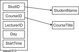
LectureOps (#(StudID, CourseId, LecturerID, Day, StartTime), StudentName, CourseTitle) |
|
StudID: Student number (unique for each student)
CourseID: Course number (unique for each course)
LecturerID: Staff number of the lecturer (unique for each lecturer)
CourseTitle: Title of the course |
|
Day and Start time identify each individual lecture session. Thus, the focus is not on the courses as such, but on the individual lecture sessions. Each tuple records that ... |
|
a student attends a specific lecture, held by a specific lecturer, on a specific day, starting at a specific time. |
|
This means that a particular lecture session and its attendance by a student are uniquely represented. The functional dependencies shown in the FD diagram apply. These are both simple functional dependencies. |
|
|
|
Figure 6.2-2: FD diagram for the relation LectureOps_1NF |
|
The redundancy arises from the fact that the name of the student and the name of the course are recorded for each course date. The reason for this is that non-key attributes (NKA; StudentName and CourseTitle) are functionally dependent on part of the key. |
|
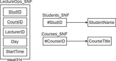
When this structural deficiency is eliminated, the redundancy-free relations shown in the following figures as FD diagrams are obtained. For the students and the courses, one new relation each is created; the original relation remains but receives foreign keys. All specified functional dependencies are full dependencies. All relations are already in 5NF (Fifth Normal Form). |
|
|
|
Figure 6.2-3: FD diagrams for the relations Lecture Operations (LectureOps_5NF), Students (Students_5NF), and Courses (Courses_5NF). |
|
6.2.2 Definition of 2NF |
|
The 2NF can thus be defined as follows: |
|
A relation is in second normal form (2NF) if every non-key attribute is fully functionally dependent on the (entire) key. |
|
Alternatively: ... if no (true) key attribute is a determinant for non-key attributes. |
|
Thus, in a relation with 1NF and without 2NF, simple functional dependencies must exist. If these are eliminated, each attribute then describes the object identified by the primary key and not another object identified by part of the key. If this condition is met, the anomalies listed above cannot occur. |
|
What has been shown above applies in principle. Relations in 1NF that are not in 2NF can be converted to 2NF. This is achieved by rearranging the attributes of the relation in different relations in such a way that a) the above 2NF condition is fulfilled and b) no information is lost in. More specifically: Each key attribute that is a determinant becomes the key of a new relation. The attributes that are functionally dependent on this key are assigned to it. The determinant itself remains in the 1NF relation, but becomes a foreign key. |
|
Compare the examples in German in |
|
- https://www.staud.info/rm2/rm_t_1.php#Abschnitt10.3 and
- https://www.staud.info/rm2/rm_t_1.php#Abschnitt10.4
|
|
6.3 Third normal form - 3NF |
|
6.3.1 Redundancy despite 2NF |
|
In very abstract terms and reduced to the essentials, the following figure illustrates the problem with relations that are not in 3NF: There is a determinant that is neither a key nor a key attribute (D in the first example, B in the second). Since such a determinant typically has several identical values, the attribute value dependent on it is recorded multiple times in C. |
|
|
|
Figure 6.3-1: 2NF and not 3NF - abstract |
|
Such "continued" functional dependencies are called transitive (see below). Relations with such a structural feature are normalized as follows: |
|
The determinant that is not a key attribute forms a new relation together with the attribute that depends on it. This determinant (which is no longer a determinant after normalization) must also remain in the original relation. There, it becomes a foreign key, thus ensuring the cohesion between the data and preventing data loss. |
|
Here are the above relations in 3NF: |
|
|
|
Figure 6.3-2: Relations in 3NF - abstract |
|
6.3.2 Example: Order headers |
|
In the previous section, the following relation resulted from the application of 2NF, which has been supplemented here with an attribute and several tuples: |
|
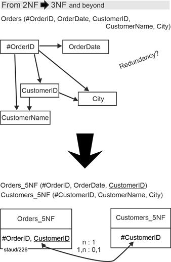
OrderHeaders (#OrderID, OrderDate, CustomerID, CustomerName, Location) |
|
This relation represents the headers of customer orders. Each tuple corresponds to one order.
OrderID uniquely identifies the order (primary key).
OrderDate records the date of the order.
CustomerID uniquely identifies the customer who placed the order.
CustomerName and City provide descriptive information about the customer. |
|
Here are some example data for the relation above: |
|
OrderHeaders_2NF |
|
| #OrderID |
OrderDate |
CustomerID |
CustomerName |
City |
| 0001 |
06/30/15 |
1700 |
Miller |
Chicago |
| 0010 |
07/01/14 |
1201 |
Sanders |
Denver |
| 0011 |
07/02/15 |
1600 |
Johnson Inc. |
New York |
| 0012 |
07/04/16 |
1900 |
Maxwell LLC |
Dallas |
| 1001 |
05/19/14 |
1700 |
Miller |
Chicago |
| 1010 |
03/20/15 |
1201 |
Sanders |
Denver |
| 1011 |
09/05/15 |
1600 |
Johnson Inc. |
New York |
| 1012 |
12/20/14 |
1900 |
Maxwell LLC |
Dallas |
| ... |
... |
... |
... |
... |
| |
OrderID: Order number
OrderDate: Date of order
CustomerID: Customer number |
|
It stores information about orders, specifically order headers and customers. The following functional dependencies apply: |
|
OrderID => OrderDate |
|
OrderID => CustomerName |
|
OrderID => CustomerID |
|
OrderID => Location |
|
CustomerID => CustomerName |
|
CustomerID => City |
|
The relation is undoubtedly in 2NF. The redundancy that still exists is due to the fact that the same customer number can of course occur very often and the customer's name and place of residence are recorded for each occurrence. The reason for this is that a non-key attribute (NKA), CustomerID, is a determinant and that there are "continuous" functional dependencies: |
|
OrderID => CustomerID => CustomerName and |
|
OrderID => CustomerID => Location |
|
The term transitive dependency is based on the corresponding term in mathematics. |
|
As a reminder (from school algebra): transitive means a relationship across another element. A and B are in some transitive relationship (rel) if the following applies: A rel C rel B. |
|
It is represented as follows: |
|
OrderID --> :: --> CustomerName |
|
OrderID --> :: --> City |
|
To eliminate this deficiency, the relation must be decomposed into two relations. The "NKA determinant" together with the functionally dependent attribute City yields the new relation Customers_5NF. |
|
The former relation loses the attribute CustomerName and retains the original determinant CustomerID as a foreign key. |
|
Customers_5NF (#CustomerID, CustomerName, City) |
|
The �old� relation loses the attribute CustomerName but retains the original determinant CustomerID as a foreign key. |
|
Orders_5NF (#OrderID, OrderDate, CustomerID) |
|
The following figure shows the entire normalization step, including the small model fragment that is created in the process. |
|
|
|
Figure 6.3-3: From 2NF to 3NF � using the example of orders/customers |
|
CustomerID: Customer number
CustomerName: Customer name |
|
6.3.3 Definition of 3NF |
|
Here is the formal version of the definitions introduced above. First, the transitive dependency: |
|
Let A, B, and C be attributes of a relation R. C is said to be transitively dependent on A, symbolically: |
|
A --->::---> C, |
|
if there is an attribute B from R for which the following applies: |
|
A => B => C (für A <> B <> C) |
|
The same applies to attribute combinations, i.e., if there are several attributes for A, B, or C. If such structures do not exist or have been eliminated, a relation is in third normal form: |
|
A relation is in third normal form (3NF) if it is in 2NF and if there are no transitive dependencies between the key and non-key attributes (NKA) (alternatively: ... if no NKA is a determinant). |
|
Thus, the following applies: |
|
- in a 3NF relation, no non-key attribute (NKA) is transitively dependent on a key, i.e., each NKA contains a property that applies to the underlying object as a whole.
- A relation is in 3NF if and only if all NKA are mutually independent and fully dependent on the key.
- "A relation R is in third normal form (3NF) if and only if, for all time, each tuple of R consists of a primary key value that identifies some entity, together with a set of zero or more mutually independent attribute values that describe the entity in some way" [Date 1990, p. 367].
|
|
This then establishes the reference to an object in the relational sense. In the FA diagram, this is expressed by arrows emanating only from the key. |
|
6.4 Boyce-Codd Normal Form - BCNF |
|
6.4.1 Redundancy despite 3NF |
|
Keys consisting of two or more attributes have already been mentioned above. They always mean that each of the attributes (e.g., EmpID and ProjName) describes an aspect of the real-world phenomenon (e.g., project employee) in an identifying manner and that together they describe the real-world phenomenon itself ("who in which project"). |
|
It sometimes happens, albeit not often, that a relation has overlapping keys. In this case, each key consists of at least two attributes (e.g., #(A,B) and #(B,C)) that have at least one attribute in common (here B). The following figure shows how this situation is expressed in an FA diagram. |
|
|
|
Figure 6.4-1: Redundancies in the 3rd normal form - 3NF and not BCNF |
|
So far, so good. If this is required by the needs of the application domain, then this is how you have to model it. Redundancies arise when there are functional dependencies between the keys, i.e., when, for example, an attribute of one key is functionally dependent on one of the other. This is also the case in reverse, since both have an identifying character as key components for a partial aspect of the phenomenon described. The following figure shows such a situation. |
|
|
|
Figure 6.4-2: Redundancies in the 3rd normal form - F.A. between key attributes |
|
For each value of A, there is a corresponding value of C. Since a certain value occurs multiple times in A (key component), the corresponding value also occurs multiple times in B. This relationship must also apply in reverse, because A and B must have key character for sub-aspects in such an arrangement. This redundancy is further increased when non-key attributes (NKA) are added to. The following figure illustrates this using the example of a single NKA. |
|
|
|
Figure 6.4-3: 3NF and not BCNF - abstract |
|
Reminder: NKA = non-key attribute |
|
With this key constellation, each NKA depends on two keys. For each multiple occurrence of an attribute value in A or C , there are also multiple entries in D. This is also redundant, even if it has not been considered in the previous steps of normalization theory. |
|
2NF and 3NF fulfilled. Despite these shortcomings, such a relation is in 2NF because there are no functional dependencies from a key attribute to an NKA, and also in 3NF because no NKA is a determinant. |
|
The solution is to move the relationship between the two attributes, which is expressed by their mutual functional dependencies, into a separate relation. In our abstract example, this creates the relation A-C. Since each value of one attribute and the other attribute occurs only once, the relationship is recorded only once. |
|
The semantics expressed by the functional dependency on the NKA is captured by a new relation with one of the "old" composite keys (it doesn't matter which one) and the NKA. In the example, this creates the relation A-B. The attribute that also occurs in the other relation from the composite key becomes a foreign key there, thus allowing the link to the other resulting relation. |
|
Finally, the BCNF |
|
|
|
Figure 6.4-4: Relations A-C and A-B in BCNF - as FA diagrams |
|
These new relations are then in Boyce-Codd Normal Form (BCNF), named after their discoverers. It also serves the purpose of optimizing the relational structure, i.e., the optimized arrangement of attributes in flat tables. |
|
It eliminates deficiencies that have been discovered over the years in relation to Codd's third normal form. Specifically, these were difficulties that arose if a relation had several composite (consisting of several attributes) and overlapping keys and if there were functional dependencies between individual key attributes. This is because 3NF does not require the full functional dependency of an attribute on the primary key if it is itself an attribute of a key. |
|
6.4.2 Example: Project Participation |
|
Let's consider the following relation to Project Participation (ProjParticipation) as an example. |
|
ProjParticipation |
|
| EmpName |
EmpID |
Role |
ProjName |
Duration |
| Stein |
12345 |
Leader |
BPR |
24 |
| Maier |
12346 |
ITSpec |
BPR |
18 |
| Müller |
23456 |
Leader |
ITIL |
18 |
| Bach |
54321 |
InfoMan |
ERP-Impl |
10 |
| Bach |
54321 |
ITSpec |
Portal |
24 |
| Bach |
54321 |
InfoMan |
SDK |
6 |
| ... |
|
|
|
|
| KA |
KA |
NKA |
KA |
NKA |
| |
Key: #(EmpName, ProjName) or #(EmpID, ProjName) |
|
Primary key: #(EmpName, ProjName) |
|
KA: key attribute, NKA: non-key attribute |
|
ERP-Impl: ERP-Implementation |
|
The following semantics apply: |
|
- The attribute EmpName is unique(!). Therefore, it can only be a small business.
- Role describes the position of the employee (Leader: project leader, InfoMan: information manager, ITSpec: IT specialist). An employees can have different roles in different projects.
- ProjName is the (unique) name of the project (e.g., BPR: Business Process Reengineering).
- Duration records the duration of project membership in months.
|
|
Textual notation: |
|
ProjParticipation (#(EmpName, (ProjName), EmpID), Role, Duration) //overlapping key |
|
The following full functional dependencies exist between the attributes: |
|
(EmpName, ProjName) => Role |
|
(EmpName, ProjName) => Duration |
|
(EmpID, ProjName) => Role |
|
(EmpID, ProjName) => Duration |
|
EmpName => EmpID |
|
EmpID => EmpName |
|
The upper part of the following figure shows the FA diagram. EmpID and EmpName are mutually functionally dependent. The relation is in 3NF because the non-key attributes are fully functionally dependent on the key and because there are no other full functional dependencies between the NKAs. |
|
Mixing of concepts |
|
Nevertheless, this relation exhibits redundancies and mixes concepts from two real-world phenomena, which leads to the anomalies already discussed. On the one hand, it records the role and project participation of employees; on the other, it records which employee ID belongs ro which person. The problem here is that the 1:1 relationship between the two key attributes EmpName and EmpID is recorded multiple times. For example, that Bach has the ID 54321. |
|
This redundancy is not eliminated by 3NF, since 3NF does not consider functional dependencies between key attributes. The anomalies in detail: |
|
- Insertion anomaly: A new employee (Dörrer) is hired and assigned an ID. However, since she is not yet assigned to a project, her data cannot be recorded (due to the requirement of entity integrity), because the key also requires a project.
- Deletion anomaly: Stein leaves the "LCD" project and his tuple is deleted. This also removes the information about his employee ID.
- Update anomaly: Bach is assigned a new employee ID. To update this information in the database, every entry of "Bach/54321" has to be changed. This violates the rule that every piece of information in the database should be stored only once.
|
|
The solution again lies in decomposing the relation: one relation ProjectParticipation, and another relation Employees (see the figure), which could, of course, be merged with an already existing Employees relation. |
|
Since the resulting relations do not exhibit the problems associated with 4NF and 5NF, the resulting relations are already in 5NF. |
|
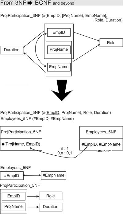
|
|
Figure 6.4-5: From 3NF to BCNF - using the example of project staff |
|
Die Relationen:
ProjParticipation_3NF (#(EmpName, (ProjName), EmpID), Role, Duration)
ProjParticipation_5NF (#(ProjName, EmpID), Role, Duration)
Employees_5NF (#EmpID, #EmpName) |
|
The lower part of the figure also contains the FA diagrams of the new relation. These once again make it clear that the achieved normal form is optimal (redundancy-free). The tabular representation finally clarifies this. The tuples that are superfluous in the new relations have been crossed out for clarification. |
|
Employees_5NF |
|
| #EmpName |
#EmpID |
| Stein |
12345 |
| Maier |
12346 |
| Miller |
23456 |
| Bach |
54321 |
| Bach
|
54321
|
| Bach
|
54321
|
| ... |
|
| KA |
KA |
| |
Key: #EmpName or #EmpID) |
|
|
|
ProjectParticipation_5NF |
|
| EmpID |
Role |
ProjName |
Duration |
| 1234 |
Manager |
BPR |
24 |
| 12346 |
DV |
BPR |
18 |
| 23456 |
Head |
ITIL |
18 |
| 54321 |
InfMan |
ERP Impl |
10 |
| 54321 |
DV |
Portal |
24 |
| 54321 |
InfMan |
SDK |
6 |
| ... |
|
|
|
| KA |
NKA |
KA |
NKA |
| |
Key: #(EmpID, ProjName) |
|
ERP-Impl: ERP-Implementation |
|
6.4.3 Definition of BCNF |
|
Relations that are in 3NF and do not exhibit any of the structural deficiencies described above are in Boyce-Codd normal form (BCNF). This can be defined as follows: |
|
A relation is in Boyce/Codd Normal Form (BCNF) if every determinant is a key (primary or secondary key). |
|
This definition also includes 2NF and 3NF. It goes further than 3NF, which only prevents an NKA from becoming a determinant. Here, a key attribute that is not itself a key is also prevented from becoming a determinant. In other words, if this definition is taken as the basis for modeling efforts, all normal forms, including BCNF, are realized. |
|
6.5 Further normal forms |
|
4NF |
|
The Fourth Normal Form concerns special cases that rarely occur in a competent design. A description in Germancan be found here: |
|
https://www.staud.info/rm2/rm_t_1.php#Kapitel13 |
|
5NF |
|
The same applies to Fifth Normal Form, which is also hardly encountered in practice. A description in German can be found here: |
|
https://www.staud.info/rm2/rm_t_1.php#Kapitel14 |
|
7 Individual/Type Pattern |
|
For a more detailed description, see https://www.staud.info/rm2/rm_t_1.php#Abschnitt15.2 (in German) |
|
|
|
7.1 The Concept |
|
The term Individual/Type describes the contrast between the perception of individual phenomena and the perception of phenomena as a whole. |
|
Other designations include: |
|
- Object/Type
- Instance/Class (in reference to object-oriented theory)
- Entity/Entity Type
- Single Object/Object Class
|
|
This pattern appears in many application domains: |
|
- Individual Animal/Animal Species
- Individual Device/Device Type
- Component/Component Type
- Individual Person/Group
- Employee/Department
|
7.2 Implementation |
|
Earlier, we showed how individual objects can be grouped into object classes. Within a class, objects share exactly the same attributes. These attributes are then managed in the database. Each attribute thus applies to all objects of the class, and each object is assigned one attribute value. |
|
However, in many application domains, there are situations where attributes must also be assigned to the class as a whole in addition to attributes for the individual objects. In such cases, attributes exist both for the individual objects and for the object class. |
|
In object-oriented theory, this pattern is captured by the so-called class attributes (see [Staud 2019, Section 2.3]). |
|
This pattern - referred to here as the Individual/Type Pattern - is ubiquitous in application domains and must therefore be reflected in data models. Unfortunately, it is often overlooked, which leads to redundancy in databases. Its foundation lies in the fact that there are objects (of various kinds) that are very similar and thus share the same attributes (animals of a genus, technical devices of a type, groups of people, etc.), but where the types, genera, or groups themselves also have attributes. |
|
Depending on the application domain and object type, the entirety of all objects is named differently in an abstract way: in general terms and referring to object-oriented theory, classes (object classes). In the case of animals, species; in the case of devices, types (device types); in the case of people, groups, etc. |
|
If you want to supplement the information of the individual objects with that of the class and simply add this to the relation with the individual information, this is redundant. Some examples: |
|
- Zoo animals. In a zoo, the individual animals (chimpanzee Eddi, orangutan Franz, elephant Paul, etc.) may be recorded by attributes, but so are the species (chimpanzees, orangutans, elephants of the species, etc.).
- Technical devices. In many contexts, individual items are recorded (cars, hard drives, aircraft spare parts, ...), while at the same time, groups of similar items are also managed (types of cars, hard drives, spare parts of a certain type, ...).
- People. In the case of humans, the individual person is often recorded (with employee numbers, names, etc.) as well as the group to which they belong (IT employees, contract workers, senior management, etc.).
|
|
When such a situation arises, there are three options: |
|
- Attributes only for individual objects. In this case, a relation is created for the objects, and the situation is resolved. This corresponds to the standard case.
- Attributes only for the class (type, genus, group). In this case, a relation is created for the class, and the matter is also resolved. Only in potential relational joins must care be taken (see examples below).
- Attributes for both individual objects and the class. In this case, two relations must be created (one for the individual objects and one for the class), and the attributes must be divided accordingly. Attributes that describe individual objects belong to the relation with instance information; attributes that describe the class as a whole belong to the relation with type information.
|
|
Thus, a database may contain both individual objects and collections of similar objects. For consistency, all such collections - regardless of whether they are called type, genus, or group in the domain - will be referred to here uniformly as types. The pattern is therefore called the Individual/Type Pattern. |
|
Example: Zoo animals - Individuals and Genera |
|
The following figure shows the pattern in an application domain involving animals, e.g., in a zoo. The animal genera in the zoo could consist of chimpanzees, orangutans, elephants, etc. For these, the relation Animal-Species is recorded with the attributes Designation (SpecName), Number of members (Count), Classification (Classif), and Notes on the type of accommodation (Housing). |
|
For the individual animals in the Animals-Individual relation, there is an animal number (AnimalID), a name (Name), the date of birth (BirthDate), the gender (sex), and the number of the building in which they are housed (BuildingID). To link the two relations, the genus designation (SpecName) is included in Animals-Individual as a foreign key. These two relations describe the situation without redundancy. |
|
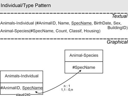
|
|
Figure 7.2-1 : Individual/Type Pattern Zoo Animals |
|
8 Gen/Spec Pattern |
|
Gen/Spec stands for Generalization/Specialization.
For more details, see [Staud 2021, Section 14.1] and https://www.staud.info/rm2/rm_t_1.php#Abschnitt15.1 (in German) |
|
|
|
8.1 The Concept |
|
Here again, the basis is objects from the application domain. In generalization/specialization, the focus is on the similarity of objects, measured by identical and specific attributes. The identical attributes are: |
|
- The key attribute
- At least one descriptive attribute
In addition to these, objects may also have specific attributes. This leads to challenges in capturing, storing, and evaluating data (see the examples below), which is why suitable solutions must be found during data modeling. |
|
Generalization as a process can be seen as grouping objects that share attributes into a higher-level entity type. |
|
Conversely, specialization can be seen as splitting a general entity type into several specialized subtypes that possess additional attributes. |
|
In relational databases, this pattern is usually implemented through multiple relations: |
|
- One for the generalization
- One for each specialization, which inherit the same key.
|
|
|
8.2 Implementation |
|
So, there are objects in application domains that share many attributes but differ in some. Consider the employees of a company. Common attributes could be: |
|
- Employee Name (EmpName), Last Name (LName), First Name (FName), Department Name (DeptName), Hiring Date (HireDate)
|
|
For Software developers, additional attributes might be relevant: |
|
- Development Environment (DevEnv), Programming Language (ProgL) (only one each, the most commonly used)
|
|
For top management, one could also record: |
|
- Remuneration Model (Remun)
|
|
How can such a pattern be handled? If all attributes are combined in a single relation, there are attributes for non-developers and non-managers that cannot be assigned ("semantically induced null entries"). This is a highly inadequate structure in attribute-based files and databases. |
|
In semantic modeling and object-oriented theory, the so-called generalization/specialization (Gen/Spec) pattern was developed to handle this. It can also be implemented in relational theory as follows: A separate relation is created for all common attributes, this is the so-called generalization , and a separate one for the attributes of the respective specialized groups, the specializations. |
|
In our example, this results in the following relations: |
|
Employees (#EmpID, LName, FName, DeptName, HireDate) |
|
Developers (#EmpID, DevEnv, ProgL) |
|
TopManagement (#EmpID, Remun) |
|
EmpID is used as the key in each case. This results in relations in which there can be an attribute value for each object and each attribute, so there is no need for semantically induced null values. |
|
An abstract example |
|
In the following example, we assume a standard situation in modeling projects: Several relations exist and suddenly it becomes apparent that they have share some attributes. Let's consider the three relations R1, R2, and R3 with the attributes listed: |
|
R1 (#A1, A2, A3, A4, A5) |
|
R2 (#A1, A2, A3, A6, A7, A8) |
|
R3 (#A1, A2, A3, A6, A9, A10) |
|
Obviously, the three relations have the attributes A1, A2, and A3 in common, while their other attributes are different. In such a case, the common attributes are placed in a separate relation, the "top-level" generalization. It will be called R4. |
|
R4 (#A1, A2, A3) |
|
This highlights another reason for Gen/Spec: a specific attribute should only appear once in the data model and then in the database, and not multiple times. R4 represents the generalization of the other three relations. These retain the key but lose the other common attributes: |
|
R1 (#A1, A4, A5) |
|
R2 (#A1, A6, A7, A8) |
|
R3 (#A1, A6, A9, A10) |
|
These three relations thus represent specializations. This data model can be expressed graphically as shown in the following figure. The graphical notation for this pattern does not have its own graphical element, as is the case with entity relationship models (ERM) and in class diagrams of object-oriented theory. It can only be recognized by the fact that the relations have the same key and by the min/max specifications between them. |
|
|
|
Figure 8.2-1: Generalization/Specialization - Abstract |
|
If you take a closer look at the textual version of this data model, you will notice that R2 and R3 have another attribute in common, R6. This requires further decomposition. The common attribute is moved to R5. R5 is then a specialization of R4 and a generalization of R2 and R3. Overall, the following applies: |
|
Generalization of all relations, "highest" generalization: |
|
R4 (#A1, A2, A3) |
|
Specialization of R4: |
|
R1 (#A1, A4, A5) |
|
Specialization of R4, generalization of R2 and R3: |
|
R5 (#A1, A6) |
|
Specializations of R5: |
|
R2 (#A1, A7, A8) |
|
R3 (#A1, A9, A10) |
|
The above text shows how the attributes are divided among the relations. The following figure clarifies the relationship between the relations. Any necessary links are made via the primary keys. If an application or query that focuses on R2 also requires the attributes of R5 and R4 or their values, they can be retrieved via relational joins. In object-oriented theory, this technique is called inheritance (the upper relation "gives" the "lower" relation its attributes when necessary). See [Staud 2019, section 6.6]. |
|
The primary keys of the generalizations and specializations are related to each other as follows: The highest generalization contains all key values. Each of its specializations contains a subset of these. This is also expressed by the cardinalities in the next figure. |
|
The cardinality is 1:1, while the min/max values are 0,1 and 1,1: not every object of the generalization must belong to a specialization, but each object of a specialization must be linked to one in the generalization. Similarly, R5 as a generalization contains all key values of R5, R2, and R3, while R2 and R3 each contain only subsets of R5. |
|
|
|
Figure8.2-2: Generalization/Specialization - Two-level and abstract |
|
Two questions remain: |
|
- Overlapping: Do the specializations overlap (i.e., do they share a non-empty subset of keys), or are they disjoint?
- Covering: Do the specializations together cover all instances of the generalization (i.e., is their union equal to the generalization), or not?
|
|
Both aspects must be taken into account, particularly for queries and evaluations, but they are not directly reflected in the data model. For a more detailed discussion in the context of object-oriented modeling, see [Staud 2019, Section 6.4]. |
|
9 Aggregation Pattern |
|
For more details, see [Staud 2021, Section 14.3] and https://www.staud.info/rm2/rm_t_1.php#Abschnitt15.3 (in German) |
|
|
|
9.1 The Concept |
|
This section deals with the pattern known in semantic data modeling and object-oriented theory as aggregation. It expresses that one object is contained in another. It does not express existence dependency - that is the task of Composition Pattern, which will be described in the next section. |
|
A typical feature of this pattern is that the contained parts have their own existence. This can be modeled in two ways: either by treating the components at the type level, or as individualized components. The following examples from the world of PCs illustrate this. |
|
9.2 Implementation |
|
First, the variant with individualized components. |
|
Application domain PCs - aggregation with individualized components |
|
Here we will focus on components that can be installed in a PC and are permanently but not inseparably connected to it (see the composition pattern in the next section). Examples include graphics cards and internal hard drives. The components are individualized, i.e., they each have a key. |
|
The following figure shows the (small) data model. There is a PC relation and a Components relation for the components. InvNr stands for inventory number. If PC and Components are the initial relations, the aggregation must be expressed by a separate PCComp relation: |
|
PCComp (#InvNoComp, InvNoPC) |
|
This allows the component to "exist" in components even if it is no longer installed in a PC. |
|
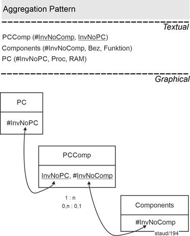
|
|
Figure 9.2-1 : Sample composition with individualized components |
|
PCComp has a structure that is surprising at first glance. Although it links PCs with their components, the attribute InvNoComp alone already has the character of a key. This is due to the individualized level: each component is unique through its inventory number InvNoComp. |
|
The data model also shows the peculiarity of the aggregation pattern: there may be components that are not assigned to any PC, and PCs that have no components (though the latter is rather unlikely). |
|
Then, the variant for the type level. |
|
Application domain PC - Components at the Type Level |
|
Here, too, the focus is on equipping each individual PC with components, but this time the components are recorded only by their designation ("graphics card xyz"), i.e., at the type level. The relation for components thus changes to: |
|
ComponentTypes (#CompName, Function) //CompName: component designation |
|
This results in the solution shown below. The aggregation is expressed by the PCComp relation as follows: |
|
PCComp (#(InvNoPC, CompName)) |
|
Thus, a PC can be associated with several components, and a component type (e.g., "IBM 123 Hard Drive") can be associated with several PCs. However, this modeling at the type level is imprecise, as the specific number of components of the same type cannot be identified in this way. If this is also to be expressed, the number (e.g., of hard drives of the "same type") must be added: |
|
PCComp (#(InvNoPC, CompName), Quantity) |
|
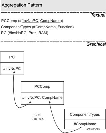
|
|
Figure 9.2-2: Aggregation Pattern with Components at the Type Level |
|
10 Composition Pattern |
|
For more details, see [Staud 2021, Section 14.4] and www.staud.info/rm1/rm_t_1.htm#Abschnitt15.4 (in German) |
|
|
|
10.1 The Concept |
|
This pattern also involves inclusion, as in aggregation, but the contained parts are inseparably connected with the higher-level whole. At least from a database perspective, and sometimes also in reality within the application domain, the contained parts are existence-dependent on the "whole": if a "whole" is deleted, its components disappear as well. |
|
10.2 Implementation |
|
This is easiest to imagine in the areas of invoicing and buildings: |
|
- If the invoice header is deleted, the invoice items also disappear.
- If the building is removed from the database, e.g., because it has been sold, the associated offices must also be removed (if they were recorded in the database).
|
|
Typical for all variants is that the key of the parent relation is inserted into the child relation as a key attribute and foreign key. |
|
Application Domain Invoicing |
|
The classic example of this pattern is the relationship between invoice headers (InvoiceHeads) and invoice items (InvoiceItems) of a given invoice. They belong inseparably together and the invoice items also disappear when the invoice is deleted from the database. |
|
This can be modeled as shown in the following example. InvoiceItems receives a composite key consisting of the invoice number (InvNo) and item number (ItemNo). InvNo is also a foreign key. |
|
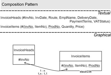
|
|
Figure 10.2-1: Composition pattern in the application domain invoicing |
|
The foreign key InvoiceItems.ProdNo indicates the need, in a comprehensive model, to describe the products in more detail using the key ProdNo. |
|
Application Domain PCs |
|
This section deals with components that are permanently connected to the PC and (normally) cease to exist with it. Examples include the WLAN component, the card reader, etc. These exist in the database and therefore have their own description, expressed by attributes. Modeling is done in such a way that the key of the parent relation PCs becomes the foreign key in the child relation Components. Since a tuple cannot exist without a foreign key entry, the entries in Components disappear when the corresponding PC is decommissioned. |
|
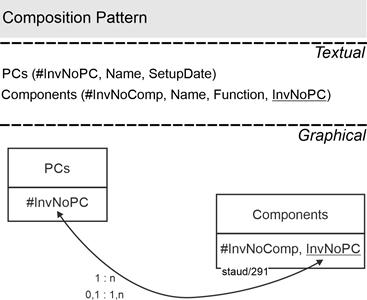
|
|
Figure 10.2-2: Composition Pattern in the PCs Application Domain |
|
11 Relationship-Attribute Pattern |
|
|
|
11.1 The Concept |
|
In Chapter 4 it was shown how, in relational databases, simple relationships - that is, relationships used to link tuples from different relations - are introduced into the data model. However, it often happens that such relationships themselves also have properties (i.e., attributes). This section shows how this is implemented in relational databases. |
|
See https://www.staud.info/Beziehungen/bz_t_1.php (in German) for a comprehensive description of relationships in databases. |
|
11.2 Implementation |
|
As always here, the solution is attribute-based. There is a relation used to establish the connection, a junction relation. To this relation, the relationship attributes are added. The implementation is as follows: a junction relation typically has a composite key, where each key attribute refers to one of the relations to be linked ("n:m", see Section 4.3). In addition to the simple linking, attributes are now added to the relationship relation. In the simplest case with two relations to be linked, this results in: |
|
RelationshipRelation (#(KA_1, KA_2), NKA_1, NKA_2, ...) |
|
KA: Key attribute, part of the key
NKA: Non-key attribute |
|
In other words, the attributes describing the relationship are simply appended to the composite key. |
|
It should be noted: The attributes to be added must describe the relationship, not the participating partners or their relations! |
|
Example: DBS and Dealers |
|
Suppose we have a database about database systems (DBS) for personal computers. One relation DBS describes the database systems, here in a simple form: |
|
DBS (#DBSName, Producer, Type) |
|
DBSName: Name of the database system
Producer: Company that developed and marketed the database system
Type: Type of the database system |
|
A second relation describes the dealers who sell database systems to end customers: |
|
Dealers (#DealerNo, Name, ZipCode, City, Street) |
|
DealerNo: Identifying number for each dealer
Name: Company name of the dealer
ZipCode: Postal code |
|
The relationship describes which dealer offers which database system, where we assume an n:m relationship. It shall be called Offer and stored in a relation of the same name: |
|
Offer (#(DBSName, DealerNo)) |
|
This version only captures the linkage: Which dealer offers which system? Typical properties of such a relationship are the market price (MPreis) and the provided service (Service): |
|
- Market price: At what price does a specific dealer offer a specific database system?
- Service: What service does a dealer provide for a specific database system?
|
|
The correct place for these two attributes is the Offer relation, which then looks like this: |
|
Offer (#(DBSName, DealerNo), MPrice, Service) |
|
MPrice: Market price
Service: Service provided by dealers |
|
These relationship attributes indeed belong to the relationship (the combination of DBS/Dealer), not to the dealer or the database system alone. |
|
- If a price were stored in the DBS relation, it would be a list price suggested by the producer.
- If Service were stored in Dealers, it would describe what service the dealer offers regardless of any specific database system.
|
|
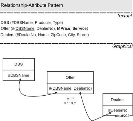
|
|
Figure 11.2-1: Relationship-Attribute Pattern in the DBS Application Domain |
|
The attributes that describe the relationship (MPrice, Service) are highlighted. |
|
12 Rules for Designing Relational Data Models |
|
Cf. [Staud 2021, Section 13.3] and www.staud.info/rm1/rm_t_1.htm#Abschnitt14.3 (in German) |
|
The following summarizes the rules for designing relational data models, as derived from the preceding discussion: |
|
- Every relation must be in 5NF. To achieve this, it is usually sufficient to bring the relation into 3NF and check whether BCNF is satisfied and whether there are any multiple multivalued attributes or incorrect join dependencies.
- Decompositions during normalization must not lead to any loss of information. This means that it must always be ensured that, through relational joins along keys and foreign keys, the information present in the original relation is preserved.
- Only attributes that are valid for all objects are included in each relation. This also follows from the normal forms, but should be made clear once again. There must therefore be no semantically induced null values. Exceptions are attributes at the beginning and end of temporal dimensions.
- Normally, there are no different relations with identical keys. Exceptions are relations within the scope of generalization/specialization and large relations with very incomplete data. In this case, a pragmatic division may be used to prevent empty entries from multiplying. An example could be a relation to database systems where you have all the "commercial" attributes but very few technical ones. Then you could split it into DBS-Commercial and DBS-Technical.
|
|
If all this is implemented, a central rule of database design is also implemented: |
|
Every piece of information (always attribute-based here) may only occur once in a database. |
|
Since in so-called SQL databases we only store attribute values of objects and relationships, the more precise formulation is the following: |
|
Each attribute value that describes an object or a relationship may only be recorded once in a database. |
|
A classic counterexample: Customers who are recorded in the database with old and previous addresses. |
|
The situation is different with NoSQL databases. For more information, see https://www.staud.info/nosql2/no_t_1.php. |
|
|
|
|
|
13 Example: Invoices |
|
|
|
13.1 Requirements Description |
|
Compare the preface to typography. |
|
It is, roughly speaking, about managing customer invoices. The system shall record invoices with their individual line items and invoice date (InvDate). Furthermore, it shall include the products (articles) appearing in those invoice items along with their quantities.
For each article, the following data are to be stored: a description, a price, and the warehouse location of the item. For customers, the system records last name (LastName), first name (FirstName), postal code (ZIP), city, street, a landline number (Landline), and a mobile number (MobilePhone). Each customer may have a maximum of two addresses stored in the database. |
|
13.2 Solution Steps |
|
Defining Relations |
|
The entities immediately recognizable as relations ("Identification + Description") are Invoices, Articles, and Customers. |
|
For invoices, we add an invoice number (InvNo) and define it as the primary key attribute. The invoice date (InvDate) is also included. However, the invoice items (positions) present a challenge. As we know, one invoice typically contains several line items - each representing one purchased article. Consequently, the items must be managed separately. We therefore divide the real-world concept Invoice into Invoice Headers (InvoiceHeaders) and Invoice Items (InvoiceItems). |
|
For the relation InvoiceHeaders, we begin with these attributes: |
|
InvoiceHeaders(#InvNo, InvDate) |
|
For Invoice Items, we introduce an item number (ItemNo). Adding such attributes is permissible and frequently necessary. We also include the article number (ArtNo) of the product appearing in this line item (always exactly one, under normal circumstances). This becomes a foreign key, providing the link to the future relation Articles (see below). Additionally, we store the quantity of that article in the line item. We do not store the article description directly within the invoice items, since (hopefully) the same article appears in multiple line items. Doing so would create redundancy and violate the Third Normal Form (3NF). |
|
Reminder:
Key: An identifying attribute or combination of attributes.
Key attribute: An attribute that is part of a key.
Non-key attribute: All remaining attributes of a relation.
Foreign key: An attribute that serves to create a relational connection. It is not a key in its own relation, but is a key in the related one.
(More on this in [Staud 2021, Section 8.2], In German) |
|
A primary key is indispensable. The item number (ItemNo) alone cannot serve as a key because it repeats across invoices. However, if we combine it with the invoice number (InvNo), the combination becomes unique. Thus, the composite key consists of (InvNo, ItemNo). The attribute InvNo contained within that key also acts as a foreign key, linking to the relation InvoiceHeaders: |
|
InvoiceItems(#(InvNo, ItemNo), ArtNo, Quantity) |
|
Notes:
- If one wishes to omit ItemNo from the key, one could instead use the article number as the second key component.
- Keys are essential. If the requirements specification fails to mention them, they must be added. |
|
The relationship between InvoiceHeaders and InvoiceItems has cardinality 1 : n, with min/max values 1,n : 1,1. This implies existence dependency - a composition. |
|
For customers, we introduce a customer number (CustNo) as the key. We add the last name, first name, and the mobile phone number, since the latter is person-specific, i.e., functionally dependent on the customer, not on an address. Hence we obtain: |
|
Customers(#CustNo, LastName, FirstName, MobilePhone) |
|
Normally, we would now add the address attributes. However, since the requirements specify more than one address per customer, the address data must be stored in a separate relation (no multiple entries within Customers!). We therefore define an address number (AddrNo) as the key: |
|
Addresses(#AddrNo, ZIP, City, Street, Landline) |
|
Landline is assigned to Addresses, because a fixed-line number is location-dependent, i.e., functionally dependent on the address. |
|
Finally, we consider the articles. The requirements specify: description, price, and warehouse location (Location). We add the previously introduced key ArtNo, yielding: |
|
Articles(#ArtNo, Description, Price, Location) |
|
At this point, the following relations exist: |
|
Addresses(#AddrNo, ZIP, City, Street, Landline) |
|
Articles(#ArtNo, Description, Price, Location) |
|
Customers(#CustNo, LastName, FirstName, MobilePhone) |
|
InvoiceHeaders(#InvNo, InvDate, ...) |
|
InvoiceItems(#(InvNo, ItemNo), ArtNo, Quantity) |
|
Remaining Relationships |
|
One important relational link has already been included: the composition between invoice headers and invoice items. The rule is: |
|
- An invoice must have at least one item.
- Each item belongs to exactly one invoice.
|
|
Thus, there exists a 1 : n relationship between InvoiceHeaders and InvoiceItems. The composite key (InvNo, ItemNo) expresses this existence dependency, since it guarantees that each invoice item must belong to one invoice header. |
|
Relationships are often not explicitly stated in requirements but must be derived from the semantics of the application domain or from methodological reasoning. |
|
Example: For the connection between invoices and customers, the semantics are: |
|
- Each invoice belongs to exactly one customer.
- A customer can have multiple invoices.
|
|
This 1 : n relationship between Customers and InvoiceHeaders (with min/max = 0,n : 1,1 or 1,n : 1,1) is implemented by adding the customer number (CustNo) as a foreign key in the relation InvoiceHeaders: |
|
InvoiceHeaders(#InvNo, CustNo, InvDate) |
|
The relationship between Articles and Invoice Items is also 1 : n: Each line item contains exactly one article, but one article may appear in several line items. The corresponding min/max values (Articles/InvoiceItems) are 0,n : 1,1. This has already been implemented by inserting ArtNo as a foreign key into InvoiceItems: |
|
InvoiceItems(#(InvNo, ItemNo), ArtNo, Quantity) |
|
Finally, the connection between Customers and Addresses remains. The requirements specify that each customer may have two addresses in the database, e.g., one billing and one delivery address. This suggests a 1 : n relationship. However, if we also consider that multiple customers may share the same address, this becomes an n : m relationship, which requires its own junction table. |
|
If we define that: |
|
- a customer exists (in the database) only if at least one address exists, and
- an address exists (in the database) only if it belongs to at least one customer,
|
|
then the min/max values (Customers/Addresses) are 1,2 : 1,m. |
|
This yields the relation Customer Addresses (CustAddr), with a composite key composed of AddrNo and CustNo: |
|
CustomerAddresses(#(AddrNo, CustNo)) |
|
Final Verification |
|
The identified relations are now complete in their final form. No further attributes need to be added - we can close the relation definitions. |
|
All relations already meet the highest normal form: each has a key and attributes that are fully functionally dependent on that key (BCNF). There are no apparent issues with 4NF or 5NF. (See also the functional-dependency diagrams below.) |
|
13.3 Solution |
|
From the preceding analysis, the following data model results. |
|
Textual Notation |
|
Addresses(#AddrNo, ZIP, City, Street, Landline) |
|
Articles(#ArtNo, Description, Price, Location) |
|
CustomerAddresses(#(AddrNo, CustNo)) |
|
Customers(#CustNo, LastName, FirstName, MobilePhone) |
|
InvoiceHeaders(#InvNo, InvDate, CustNo) |
|
InvoiceItems(#(ItemNo, InvNo), ArtNo, Quantity) |
|
Graphical Notation |
|
The question of whether all relationships have truly been implemented is answered most clearly by the graphical representation of the data model. |
|
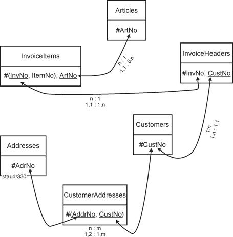
|
|
Figure 13.3-1: Relational data model |
13.4 Functional-Dependency (FD) Diagrams |
|
Brief notes on functional-dependency diagrams were given earlier; a comprehensive introduction can be found in [Staud 2021, Chapter 8] and at http://www.staud.info/rm1/rm_t_1.htm#Kapitel9, both in German. |
|
Examining the functional dependencies of the relations is highly beneficial. Such diagrams make it particularly clear whether the relations indeed satisfy the highest normal form. |
|
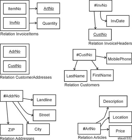
|
|
Figure 13.4-1: FD diagrams for the relations of the data model |
14 Implementation with MySQL |
|
Here, MySQL is used under XAMPP. To follow the examples, you therefore need to download XAMPP and then start Apache and MySQL: |
|

|
|
|
|
This then makes it possible to start phpMyAdmin with any browser using the command
http://localhost/phpmyadmin: |
|
|
|
|
|
The SQL window will be used in the following sections. The directory in the left column displays the databases that have been created. See also the appendix. |
|
SQL and Case Sensitivity |
|
SQL commands are not case sensitive. This means you can write your statements in uppercase, lowercase, or a mix of both - for example, |
|
SELECT * FROM customers; and select * from customers; work exactly the same way. |
|
However, this rule applies only to SQL keywords and parameters, not to the data itself. Text values stored in tables, such as names or addresses, are treated as they are. So "Smith" and "smith" are considered different. |
|
|
|
14.1 Task |
|
The task could be formulated as follows: |
|
- Create the database for the above data model using SQL commands.
- Insert demo data that makes the relationships visible.
- Then execute queries, including those that traverse the relational connections.
|
|
14.2 Solution |
|
Creating the Database and Relations |
|
The database shall be named InvCu (Invoices / Customers). Some attribute names are shortened slightly for convenience. |
|
Important: When executing the SQL commands manually, always pay attention to the order of creation! When relationships exist, create the relation with the primary key first, followed by the one that contains the foreign key. |
|
The following command creates the database: |
|
|
CREATE DATABASE invcu DEFAULT CHARACTER SET latin1 COLLATE latin1_german1_ci;
|
|
To set up your own database:
Copy and paste the command into the SQL window and execute it. |
|
And now the relations: |
|
Relation Customers |
|
Customers(#CustNo, LastName, FirstName, MobilePhone) |
|
|
CREATE TABLE customers (CustNo SMALLINT(5), LastName CHAR(10), FirstName CHAR(10), MobilePhone CHAR(12), PRIMARY KEY (CustNo));
|
|
To set up your own database:
Select the InvCu database.
Copy and paste the command into the SQL window and execute it. |
|
The structure of the relation can be displayed with the command describe customers: |
|
|
|
Relation Articles |
|
Articles(#ArtNo, Description, Price, Location) |
|
|
CREATE TABLE articles (ArtNo SMALLINT(4), Description VARCHAR(10), Price DECIMAL(7,2), Location CHAR(5), PRIMARY KEY (ArtNo));
|
|
To set up your own database:
Copy and paste the above command into the SQL window and execute it. |
|
|
describe articles
|
|
|
|
Relation Addresses |
|
Addresses(#AddrNo, ZIP, City, Street, Landline) |
|
|
CREATE TABLE addresses (AddrNo SMALLINT(7), ZIP CHAR(5), City CHAR(10), Street CHAR(10), Landline CHAR(15), PRIMARY KEY (AddrNo));
|
|
To set up your own database:
Copy and paste the above command into the SQL window and execute it. |
|
|
describe addresses
|
|
|
|
Relation InvoiceHeaders |
|
InvoiceHeaders(#InvNo, InvDate, CustNo) |
|
|
CREATE TABLE InvoiceHeaders ( InvNo SMALLINT(6), CustNo SMALLINT(5), InvDate DATE, PRIMARY KEY (InvNo), FOREIGN KEY (CustNo) REFERENCES customers(CustNo));
|
|
To set up your own database:
Copy and paste the above command into the SQL window and execute it. |
|
describe invoiceheaders |
|
|
|
Relation InvoiceItems |
|
InvoiceItems(#(InvNo, ItemNo), ArtNo, Quantity) |
|
|
CREATE TABLE InvoiceItems (InvNo SMALLINT(6), ItemNo TINYINT(3) UNSIGNED, ArtNo SMALLINT(4), Quantity SMALLINT(2),
|
|
|
PRIMARY KEY (InvNo, ItemNo),
|
|
|
FOREIGN KEY (ArtNo) REFERENCES articles(ArtNo),
|
|
|
FOREIGN KEY (InvNo) REFERENCES InvoiceHeaders(InvNo)
|
|
|
);
|
|
To set up your own database:
Copy and paste the above command into the SQL window and execute it. |
|
|
describe invoiceitems
|
|
|
|
Relation: CustomerAddresses |
|
CustomerAddresses(#(AddrNo, CustNo)) |
|
|
CREATE TABLE CustomerAddresses (
|
|
|
AddrNo SMALLINT(7),
|
|
|
CustNo SMALLINT(5),
|
|
|
PRIMARY KEY (AddrNo, CustNo),
|
|
|
FOREIGN KEY (CustNo) REFERENCES customers(CustNo),
|
|
|
FOREIGN KEY (AddrNo) REFERENCES addresses(AddrNo)
|
|
|
);
|
|
To set up your own database:
Copy and paste the above command into the SQL window and execute it. |
|
|
describe customeraddresses
|
|
|
|
14.3 Inserting Data |
|
Relation Customers |
|
|
INSERT INTO customers (CustNo, LastName, FirstName) VALUES (1007, 'Aberer', 'Anton');
|
|
|
INSERT INTO customers (CustNo, LastName, FirstName) VALUES (1008, 'Blauer', 'Giuseppe');
|
|
|
INSERT INTO customers (CustNo, LastName, FirstName) VALUES (1009, 'Caeser', 'Filippa');
|
|
|
INSERT INTO customers VALUES (1010, 'Dodolo', 'Rita', '1234567890');
|
|
|
INSERT INTO customers VALUES (1011, 'Steiner', 'Sepp', '2345678901');
|
|
To set up your own database:
Copy and paste the above command into the SQL window and execute it.
If repetition is necessary due to an error: Start with DELETE FROM customers; |
|
Resulting relation: |
|
|
SELECT * FROM customers;
|
|
| #CustNo |
LastName |
FirstName |
MobilePhone |
| 1007 |
Aberer |
Anton |
NULL |
| 1008 |
Blauer |
Giuseppe |
NULL |
| 1009 |
Caeser |
Filippa |
NULL |
| 1010 |
Dodolo |
Rita |
1234567890 |
| 1011 |
Steiner |
Sepp |
2345678901 |
| |
The key designation has been added. |
|
Relation Addresses
|
|
|
INSERT INTO addresses (AddrNo, ZIP, City, Street) VALUES (1001, '32801', 'Orlando', '15 Oak St');
|
|
|
INSERT INTO addresses (AddrNo, ZIP, City, Street) VALUES (1011, '80202', 'Denver', '92 Main Rd');
|
|
|
INSERT INTO addresses VALUES (2011, '98101', 'Seattle', '8 Pine Ave', '111-2222');
|
|
Resulting relation: |
|
|
select * from addresses;
|
|
| #AddrNo |
ZIP |
City |
Street |
Landline |
| 1001 |
32801 |
Orlando |
15 Oak St |
NULL |
| 1011 |
80202 |
Denver |
92 Main Rd |
NULL |
| 2011 |
98101 |
Seattle |
8 Pine Ave |
111-2222 |
| |
The key designation has been added. |
|
Relation CustomerAddresses
|
|
|
INSERT INTO CustomerAddresses VALUES (1001, 1007);
|
|
|
INSERT INTO CustomerAddresses VALUES (2011, 1007);
|
|
|
INSERT INTO CustomerAddresses VALUES (1001, 1008);
|
|
|
INSERT INTO CustomerAddresses VALUES (1011, 1009);
|
|
|
INSERT INTO CustomerAddresses VALUES (2011, 1010);
|
|
To set up your own database:
Copy and paste the above command into the SQL window and execute it.
If repetition is necessary due to an error: Start with DELETE FROM customerAddresses; |
|
Resulting relation: |
|
|
SELECT * FROM customeraddresses;
|
|
| AddrNo |
CustNo |
| 1001 |
1007 |
| 1001 |
1008 |
| 1011 |
1009 |
| 2011 |
1007 |
| 2011 |
1010 |
| |
#(AdrNo, CustNo) |
|
Key and foreign keys have been added. |
|
|
|
Side Note: Linking Customers and Addresses - Does it work as designed? |
|
|
SELECT c.CustNo, c.LastName, c.FirstName, c.MobilePhone, a.AddrNo, a.ZIP, a.City, a.Street
|
|
|
FROM customers c, addresses a, CustomerAddresses ca
|
|
|
WHERE c.CustNo = ca.CustNo AND a.AddrNo = ca.AddrNo;
|
|
Customers and their adresses |
|
| CustNo |
LastName |
FirstName |
MobilePhone |
AddrNo |
ZIP |
City |
Street |
| 1007 |
Aberer |
Anton |
NULL |
1001 |
32801 |
Orlando |
15 Oak St |
| 1008 |
Blauer |
Giuseppe |
NULL |
1001 |
32801 |
Orlando |
15 Oak St |
| 1009 |
Caeser |
Filippa |
NULL |
1011 |
80202 |
Denver |
92 Main Rd |
| 1007 |
Aberer |
Anton |
NULL |
2011 |
98101 |
Seattle |
8 Pine Ave |
| 1010 |
Dodolo |
Rita |
1234567890 |
2011 |
98101 |
Seattle |
8 Pine Ave |
| |
#(CustNo, AddrNo) |
|
The table shows that it worked as expected. |
|
End of side note. |
|
|
|
Relation Articles |
|
|
INSERT INTO articles VALUES (100, 'Gamer-PC', 2500.00, 'ST007');
|
|
|
INSERT INTO articles VALUES (101, 'Office-PC', 1200.00, 'ST018');
|
|
|
INSERT INTO articles VALUES (102, 'Developer-PC', 3200.00, 'ST100');
|
|
To set up your own database:
Copy and paste the above command into the SQL window and execute it.
If repetition is necessary due to an error: Start with DELETE FROM articles; |
|
Result: |
|
|
select * from articles;
|
|
| #ArtNo |
Description |
Price |
Location |
| 100 |
Gamer-PC |
2500.00 |
ST007 |
| 101 |
Office-PC |
1200.00 |
ST018 |
| 102 |
Developer- |
3200.00 |
ST100 |
| |
The key designation has been added. |
|
Relation InvoiceHeaders
|
|
|
INSERT INTO InvoiceHeaders VALUES (23001, 1007, '2023-03-27');
|
|
|
INSERT INTO InvoiceHeaders VALUES (23010, 1009, '2023-05-20');
|
|
To set up your own database:
Copy and paste the above command into the SQL window and execute it.
If repetition is necessary due to an error: Start with DELETE FROM InvoiceHeaders; |
|
Result: |
|
|
SELECT * FROM invoiceheaders;
|
|
| #InvNo |
CustNo |
InvDate |
| 23001 |
1007 |
2023-03-27 |
| 23010 |
1009 |
2023-05-20 |
| |
The key and foreign key designation has been added. |
|
Relation InvoiceItems
|
|
|
INSERT INTO InvoiceItems VALUES (23001, 1, 100, 1);
|
|
|
INSERT INTO InvoiceItems VALUES (23001, 2, 101, 2);
|
|
|
INSERT INTO InvoiceItems VALUES (23001, 3, 100, 1);
|
|
|
INSERT INTO InvoiceItems VALUES (23010, 1, 101, 3);
|
|
|
INSERT INTO InvoiceItems VALUES (23010, 2, 102, 1);
|
|
To set up your own database:
Copy and paste the above command into the SQL window and execute it.
If repetition is necessary due to an error: Start with DELETE FROM InvoiceItems; |
|
Result: |
|
|
SELECT * FROM invoiceitems;
|
|
| InvNo |
ItemNo |
ArtNo |
Quantity |
| 23001 |
1 |
100 |
1 |
| 23001 |
2 |
101 |
2 |
| 23001 |
3 |
100 |
1 |
| 23010 |
1 |
101 |
3 |
| 23010 |
2 |
102 |
1 |
| |
#(InvNo, ItemNo) |
|
The key and foreign key designation has been added. |
|
14.4 Example Queries |
|
Task 1
|
|
List all invoices with their invoice-relevant data. Avoid duplicate attributes resulting from key/foreign-key overlap. Sort ascending by invoice number and item number. |
|
Solution: |
|
|
SELECT ih.InvNo, ih.CustNo, ih.InvDate, ii.ItemNo, ii.ArtNo, ii.Quantity, a.Description, a.Price
|
|
|
FROM InvoiceHeaders ih, InvoiceItems ii, articles a
|
|
|
WHERE ih.InvNo = ii.InvNo AND ii.ArtNo = a.ArtNo
|
|
|
ORDER BY ih.InvNo, ii.ItemNo;
|
|
|
|
| InvNo |
CustNo |
InvDate |
ItemNo |
ArtNo |
Quantity |
Description |
Price |
| 23001 |
1007 |
2023-03-27 |
1 |
100 |
1 |
Gamer-PC |
2500.00 |
| 23001 |
1007 |
2023-03-27 |
2 |
101 |
2 |
Office-PC |
1200.00 |
| 23001 |
1007 |
2023-03-27 |
3 |
100 |
1 |
Gamer-PC |
2500.00 |
| 23010 |
1009 |
2023-05-20 |
1 |
101 |
3 |
Office-PC |
1200.00 |
| 23010 |
1009 |
2023-05-20 |
2 |
102 |
1 |
Developer- |
3200.00 |
| |
Task 2
|
|
Create a list of all customers with their addresses, again without redundant attributes from key/foreign-key repetition. |
|
Solution |
|
|
SELECT c.CustNo, c.LastName, c.FirstName, c.MobilePhone, a.ZIP, a.City, a.Street, a.Landline
|
|
|
FROM customers c, addresses a, CustomerAddresses ca
|
|
|
WHERE c.CustNo = ca.CustNo AND ca.AddrNo = a.AddrNo;
|
|
|
|
| CustNo |
LastName |
FirstName |
Mobile-Phone |
ZIP |
City |
Street |
Landline |
| 1007 |
Aberer |
Anton |
NULL |
32801 |
Orlando |
15 Oak St |
NULL |
| 1008 |
Blauer |
Giuseppe |
NULL |
32801 |
Orlando |
15 Oak St |
NULL |
| 1009 |
Caeser |
Filippa |
NULL |
80202 |
Denver |
92 Main Rd |
NULL |
| 1007 |
Aberer |
Anton |
NULL |
98101 |
Seattle |
8 Pine Ave |
111-2222 |
| 1010 |
Dodolo |
Rita |
1234567890 |
98101 |
Seattle |
8 Pine Ave |
111-2222 |
| |
15 Appendix - Information from MySQL about the Database |
|
|
|
15.1 The Data Model of the MySQL Database "ReCu" |
|
When you click the Designer button in the horizontal toolbar at the top of the window, the diagram shown below appears. It provides a clear overview of the participating relations, their attributes, and the connections between them. The data types of all attributes are also displayed. |
|
This view can be very helpful in many situations, especially when troubleshooting - for instance, if the data types of a key and its corresponding foreign key do not match. |
|
|
|
Abbildung 15.1-1: MySQL view of the relational data model Invoices |
|
15.2 List of the Relations |
|
|
|
Abbildung 15.2-1: List of the relations in a database with some of their characteristics. |
|
These two figures give us a small impression of what is called the data dictionary. It contains comprehensive information about all elements of the database and its structure. |
|
|
|
|